Chapter 4: Hedging the Wings

Here, we explore practical ways to hedge against ruin, at relatively low cost. We focus on the short 1×2 ratio spread on equity indices and bonds and the short VIX futures, long VIX calls strategy. Both are designed to provide powerful extreme event protection while collecting premium or benefitting from roll down. Naturally, there are subtleties to every trade that can only be learned by experience. However, this chapter should provide a rough road map to hedging equity and interest rate risk. The structures in this chapter should be broadly applicable to any market where the implied volatility skew moves in a predictable way during a crisis.

TAKING THE OTHER SIDE OF THE 1×2

Hedging the “wings” conjures up the bizarre image of the market return distribution as some sort of bird, a phoenix rising from the ashes, perhaps. Nonetheless, the phrase is widely used. The wings refer to the extremes of the distribution. If the 1×2 is so dangerous, why not turn it on its head? Selling the 1×2 is an inexpensive way to isolate the put skew in advance of a crisis. This is not to say that we want to short a ratio spread with the same strikes as the Batman trade in Chapter 3. For extreme event hedging, we typically target lower deltas than the Batman trade does, as we want to profit from a significant repricing of extreme event risk. The hedge is not really concerned with moderate moves in the spot. Figure 4.1 pushes our deltas further out along the put skew. 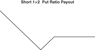Figure 4.1 Payout at maturity for short put ratio strategy

We track the performance of a strategy that sells 25 delta puts and buys 10 delta puts in a 1:2 ratio. The underlying index is the S&P 500. The position is rolled weekly, to re-establish a delta-neutral position.

COMPARING THE 25 AND 10 DELTA PUTS

If we want to build hedging structures, we need to start by identifying rich and cheap points on the skew. We can then buy relatively cheap strikes, while avoiding or even selling the expensive ones. One way to approach the problem is to look for persistent anomalies. Is there excess demand for specific levels of protection? The following analysis suggests that investors have historically overpaid for insurance against moderate moves in the S&P 500, in absolute and relative terms. As we discussed in the introduction, –20% moves seem implausible until the first –10% drop. Investors also do not seem to embrace the idea that you can make a significant amount of money on an option without the spot ever reaching the strike. For a strategy where you do not hold to maturity, what is really needed is a re-pricing of risk across different strikes.

The following example is quite simple but illustrates our point. The results are summarised in Table 4.1. Using roughly 10 years of historical data (ranging from mid-2005 to mid-2015), we have compared the performance of a rolling strategy in 4-week S&P 500 puts, for a range of deltas. We have chosen 10, 25 and 40 delta puts and rolled them weekly. This covers a fairly broad and representative range of strikes and we can be reasonably assured that the implied volatility of each option will be accurate. We have made the simplifying assumption that there is always a “flex” 4 week put with the correct delta. The flex feature allows you to specify the strike and maturity date of the option you wish to trade. We have calculated the Black–Scholes price of the puts using an interpolated implied volatility and repriced them after a week, before reloading into a fresh 4-week put. The “interpolated” number is a weighted average of implied volatilities for traded options with nearby maturities and strikes. We have also normalised the returns of each put strategy so that their volatilities match. If a given week is bullish or uneventful, the price of each put will drop. The 10 delta strategy will benefit the most from a volatility spike, as the skew will have likely steepened. The weekly return is based on the change in the option price divided by the index value at the beginning of the week.

Table 4.1 Historical performance of S&P puts with variable deltas (volatility-adjusted)

| | 10 delta put | 25 delta put | 40 delta put || --- | --- | --- | --- || average weekly return | –0.053% | –0.083% | –0.087% |

It's worth paying a bit more attention to the 25 and 10 delta puts (Figure 4.2). These are in the area where we want to hedge. Having matched their realised volatility, it's apparent that they perform similarly during the worst 1-week drops in the index. 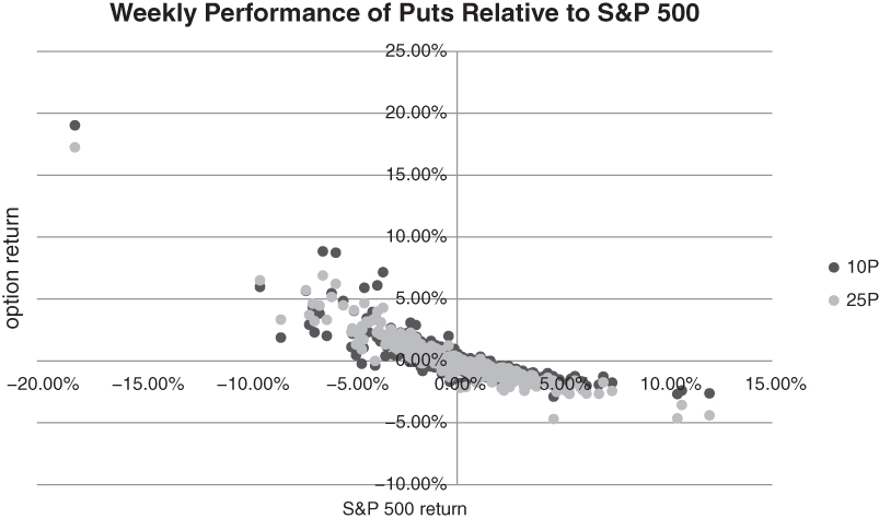Figure 4.2 10 delta S&P puts offer more “bang for the buck”

The 10 delta puts rarely wind up in the money, but benefit from rising volatility and skew steepening if the index drops sufficiently. We re-emphasise that deep OTM puts do not have to land in the money to “pop” in your favour. The spot price doesn't need to drop below the strike. Their value simply needs to be re-assessed by the market. Note that we have bought roughly 1.5 times as many 10 delta puts as 25 delta puts, so that the strategies have the same historical volatility. If we track the performance of each delta over time, it becomes apparent that the volatility-adjusted 10 delta puts outperform in quiet markets, yet provide similar levels of protection during extreme market conditions (Figure 4.3). 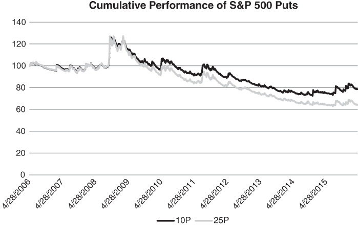Figure 4.3 Relative performance of 4-week 10 and 25 delta puts, constant risk budget

The 25 delta put strategy requires a greater premium outlay, yet doesn't do much more for you. Superficially, it might look a bit better, as you can tell your clients that you have made something when the S&P drops by a small amount. That's about it. Once you conclude that the 10 delta put is the superior hedging instrument, you can explore structures where you sell a small number of 25 delta calls and buy a larger number of 10 delta calls. When you sell the 25 delta, 10 delta put spread in a 1:1 ratio, you are trying to extract alpha from the market. Overbuying the 10 delta put converts your alpha trade into a hedge, while retaining some of the attractive features of a short put spread. In particular, it offers significant protection at low cost. In many instances, you can even collect to put the trade on, as we see below. Buying and selling an unequal number of puts with two different strikes generates something called a ratio spread. When you overbuy options at the wing, convention dictates that you are short the 1×2. This convention suggests that investors are more inclined to buy 1×2s than sell them. The payout at maturity for the short 1×2 looks a bit like a square root operator, so “square root hedge” is a convenient mnemonic for the strategy. The analysis that follows assumes that we have sold 1,000 1×2 put ratios on the Euro Stoxx 50 index, with roughly 40 days to maturity. Specifically, we have sold 1,000 25 delta puts and bought 2,000 10 delta puts at the point of entry. Note that Euro Stoxx 50 options have a multiplier of 10 Euros.

Before we analyse the short 1×2 in more detail, we provide further evidence that the 25 and 40 delta puts are to be avoided. In this instance, we take a regime-specific approach. The easiest way to split the data is to think of 2008 as a “high risk” scenario and everything else as normal. We'll be politically correct and emphasise that the high risk scenario is not “abnormal” in any way. It can't be expunged from the data. We can then tabulate the historical performance of the 10, 25, 40 and 50 delta puts as a percentage of premium paid.

On a historical basis, all of the above options appear to be expensive. There is no silver bullet in terms of cost. However, some may be more expensive than others. Relatively speaking, the 10 delta put offers decent value. The bar chart allows us to visualise where the market implied distribution might be mispriced. In particular, the market seems to be overestimating the probability of a moderate drop in the index. Very small and very large drops are priced more reasonably. Figure 4.4 serves to clarify things.

The implied distribution is relatively Gaussian, though not exactly so. To some extent, the options market does account for large downside jumps. For equity indices, the implied volatility skew predicts that left-tail events will occur somewhat more frequently than a normal distribution would suggest. However, our analysis suggests that left-tail events are still underpriced relative to “typical” down moves. Selling deep OTM options is attractive to investors who have no experience or memory of the last face-ripping sell-off and this compresses the put skew. We need to depart even further from a classic bell curve if we want to accurately represent the data. 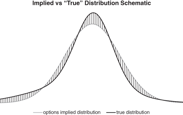Figure 4.4 Our view on the differential between “true” returns and those implied by the skew

We want to avoid buying puts or put spreads where the shaded area is above the black line, while focusing on areas where the excess demand for hedging is relatively low.

In the high risk 2008 scenario, it is fairly clear that lower delta puts generate larger returns, as a percentage of initial premium paid. High delta puts don't provide much extreme event protection, relative to their cost. Obviously, you can buy a larger number of 10 than 50 delta puts on a fixed budget. This can pay dividends in a severe crisis.

To an extent, Figure 4.5 confirms what we have been saying all along. As shown, 25 delta puts on equity indices are expensive. The same analysis applies broadly to other risky assets, such as carry currencies. There are enough instances where 25 delta puts wind up in the money that we can say this with confidence. These are the sort of puts that large institutions like to hold as protection against “realistic” downside scenarios. We can draw another conclusion from Figure 4.5. Buying 1 50 delta put and selling 2 25 delta puts (the left half of the Batman) seems reasonable as an alpha play, if you can guard against extreme event risk. However, selling the 25 delta put and buying 2 10 delta puts has even greater utility in a portfolio context. You wind up with a position that is long extreme event risk, while selling an expensive put along the skew. 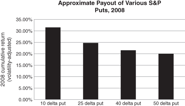Figure 4.5 Punchiness of volatility-adjusted returns for various deltas, 2008

Some managers have argued that a rolling OTM put strategy is a decent benchmark for an equity hedging overlay. The 25 delta put is a natural choice when constructing a benchmark, as it's “half way” between an ATM and 0 strike put in a probabilistic sense. It's also a benchmark that no one in their right mind would want to hold for an extended period of time. Rolling 25 delta puts consistently loses money and even mega-events such as the 2008 crisis are not enough to overcome the severe negative carry. Hedging overlay managers would be incentivised to do very little hedging at all if beating the benchmark were the only goal. Leave the patient alone. Virtually any strategy that isn't too invasive will beat the 25 delta put benchmark over the long term.

We can only conclude that benchmarking an equity protection strategy is still an open question. Our view is that hedging adds substantial value if it can roughly break even over a complete market cycle while offering considerable protection during a systemic crisis. This idea is linked to the notion of “crisis alpha”, which we will explore in Chapter 6. Crisis alpha strategies promise a bit more than what we have described above. In particular, they try to break even during quiet markets, with outperformance in high volatility periods. This is a difficult target, as performance would then be materially positive over a market cycle.

When discussing the merits of a particular structure, we find ourselves moving back and forth between historical performance charts and scenario-based payout curves. Coming to grips with the potential range of outcomes is crucial for someone who wants to manage risk on a day-to-day basis. In Figure 4.6, we graph the “square root” payout of the short 1×2 at maturity. 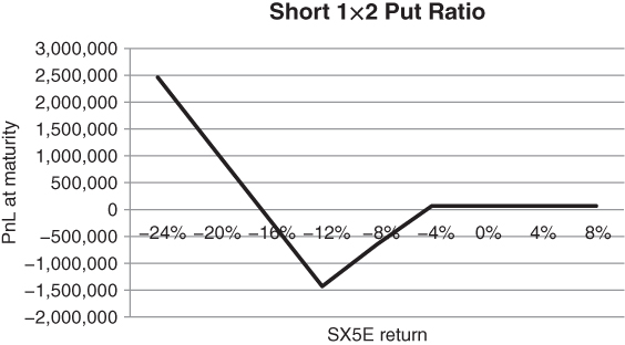Figure 4.6 Profit/loss at maturity for a short 1×2 put ratio on the SX5E index

The payout curve is derived from 4% and 12% OM strikes, on the Euro Stoxx 50 index. As above, we assume that we have sold 1,000 1×2 put ratios. Is it worth holding the structure to maturity? After all, the square root payout does have some attractive features. Since you are a premium collector in this example, you actually make money if the index has dropped less than –4% at expiration. Your profit also crosses 0 and increases linearly as the index drops more than –16%. The trouble is that the hedge actually loses a substantial amount if the index takes a hit in the –10% range, but does not collapse. Moderate down moves are the price you have to pay for the short 1×2. Naturally, you have the option of rolling the structure if it quickly goes in the money. Then you don't have to worry too much about the deep trough in the payout curve at expiration, as Figure 4.7 suggests. We cover a range of instantaneous moves from –24% to +8%, in an attempt to show how much gamma is embedded in the short 1×2. It's worth mentioning that some intriguing trades along these lines did crop up in 2008 and 2009. As equity indices collapsed, several short S&P 500 put ratios went through the market with strikes that seem incredible today. One structure revolved around selling puts with a strike around 700 and over-hedging with puts in the 500 range! In that event, the S&P 500 would have truly lived up to its name. While this sort of structure seemed bizarre at the time, it allowed the buyer to collect a premium while hedging against a Great Depression-type scenario. 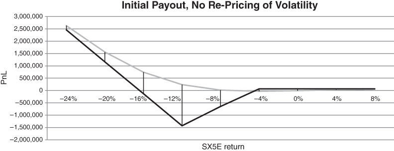Figure 4.7 Payout of short 1×2, constant volatility assumption

At first sight, the strategy only seems to hedge very extreme events, at almost unreachable levels. The payout curve doesn't slingshot in your favour until the index drops about –10% intraday. At –10%, trading is likely to be halted on a broad-based index. If the curve is correctly specified, this means that there is virtually no scenario under which you can realise a profit on day 1. As time goes by, you then face severe time decay unless the index recovers or collapses completely.

However, our analysis to this point is incomplete. We are missing something crucial. In particular, we have not properly incorporated the role of vega when repricing the structure. For a structure such as this, vega is our friend. If the SX5E goes into free fall over a 1-week horizon, implied volatility is likely to spike violently. This should have a disproportionate impact on the original 10 delta put. In volatility units, the 10 and 25 delta strikes have moved closer together, so the position behaves more like a long put at the original 10 delta strike. In Figure 4.8, we assume that a week has passed. We assume a level 20-point shift in implied volatility, unconditional on the index return. 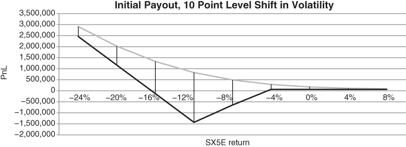Figure 4.8 Payout of short 1×2, volatility “jacked up” by 20 points

The hedge really starts to kick in at around –4%. If the SX5E drops by –8% in a week, the hedge makes roughly +2% at the index level. Extrapolating along the curve, if there is a really severe –16% collapse in the SX5E, the hedge makes nearly +5% at the index level. We have cut off a significant amount of downside using a strategy that collects premium at the outset. It is also worth mentioning that these estimates are conservative, as there is another factor that can work in our favour during a risk event. As volatility rises, the put skew is likely to steepen and our structure is manifestly long the skew. Implied volatility at the 10 delta strike will increase disproportionately to the 25 delta strike, giving us an extra performance kicker.

It's instructive to see how our short 1×2 put ratio would have done in the past, as proof of concept. Our mindset is changing from that of a discretionary options trader who wants to understand the range of outcomes for a specific structure to that of a systematic investor. Here, we want to check whether repeating the same strategy over and over again would have worked in the past. Our running hypothesis is that moderately OTM puts are overpriced relative to far OTM ones. This is based on excess demand for puts that cover “reasonable” scenarios. It is not immediately apparent whether options that are far OTM are rich or cheap. However, when combined with the statistically overpriced options, it is possible to construct extreme event hedges that are not too expensive. We analyse historical performance and the payoff curve for these structures. The following study is a direct consequence of our previous studies. We have tracked the performance of a short 1×2 put ratio on the S&P 500 over a 10-year window. Specifically, we sold 1 25 delta put and bought 2 10 delta puts, resetting the structure weekly. Both strikes had 4 weeks to maturity at initiation. Our results are summarised in Figure 4.9. 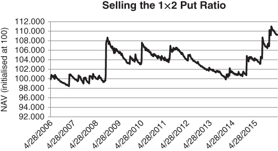Figure 4.9 Historical performance of short 1×2 on the S&P 500, gross of costs

By “NAV”, we mean the hypothetical net asset value of the strategy. The short 1×2 is a surprisingly good hedge if transacted cheaply and correctly. It more than breaks even over a 10-year historical window, while providing significant protection during volatility spikes such as the Lehman crisis and the “flash crash” of May 2010. The average premium outlay for the short 1×2 was 6 basis points per week, or roughly 3.1% per year. This compares favourably to a rolling position in 10 delta puts, which cost roughly 26.3% per year.

The cost reduction is enormous, given that you have completely blocked out the extreme downside for the index. Yet for many money managers, hedging with short 1×2s is unpalatable. They simply do not like the idea of losing money on a hedge when the index drifts down, compounding the loss in their long portfolio. This may be the reason why short 1×2s with low delta strikes have tended to be attractively priced over time. The only players who typically like to hold short put and call ratios are market makers, as they want to hold low delta options to reduce the risk of going bankrupt.

We acknowledge that realised returns would have been a bit lower than the ones in the chart above, as we have not accounted for transaction costs. At first glance, rolling 1×2s every week must be expensive and might offset the benefits of the trade. Experience suggests that rolling costs can be kept at a reasonable level if we have competitive brokerage terms and restrict ourselves to the largest and most liquid markets. Our purpose here is not to “give away the shop”, but rather to show how interesting and unorthodox hedging structures can be derived from long-term back-tests. One might argue that our back-test doesn't overwhelmingly favour the 10 delta put. The short 1×2 strategy returns are only mildly positive and require intermittent spikes in volatility to stay positive. If there is a long quiet spell, the strategy will not be able to overcome negative drift. Once we broaden our perspective, however, the 10 delta put becomes more compelling. We tabulate the average cost of 10, 25, 40 and 50 delta puts with 1 month to maturity below. Our reference index is the S&P 500, as before. Note that we have overbought the 10, 25 and 40 delta puts so that their in-sample volatility matches the 50 delta put.

The volatility-adjusted 10 delta puts are the cheapest. But do they offer comparable protection, given their cost? Using 2008 as a reference, the answer is yes, according to the following chart.

In a low-volatility regime, the short 1×2 put ratio acts as a particularly powerful hedge. It offers excellent protection against a “flash crash”, such as the one witnessed in May 2010. It benefits from acceleration in the spot toward the 10 delta strike as well as dramatic steepening in the put skew. The short 1×2 is also an efficient way to protect against a geopolitical event that may occur in an otherwise benign market. This is where most of the extreme convexity on the rightside of the graph is observable. Figure 4.10 only considers cases where the VIX was below 20 before the structure was initiated. 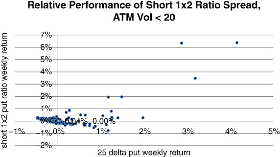Figure 4.10 Convex payout of short 1×2 when initiated in low volatility regime

It is reasonable to ask why the volatility-adjusted short 1×2 offers more bite in relatively quiet market regimes. This is largely a function of the distance between the 25 and 10 delta strikes. When volatility is low, the two strikes are bunched close together. Any lurch down in the index will bring the 10 delta put in play, immediately creating a geared downside payout on the index. We measure the sensitivity of the strike distance to ATM volatility in Figure 4.11. 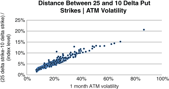Figure 4.11 Distance between strikes in 1×2 increases in tandem with ATM volatility

The strike distance is almost linearly dependent on ATM volatility. However, skew effects create some dispersion around the line of best fit. If the skew is a bit steeper than expected for a given level of ATM implied volatility, the 25/10 distance will be a bit larger than usual.

It's worth checking that the short 1×2 put ratio works for other equity indices as well as shown in Figure 4.12. Here, we track historical performance for the FTSE 100 index. 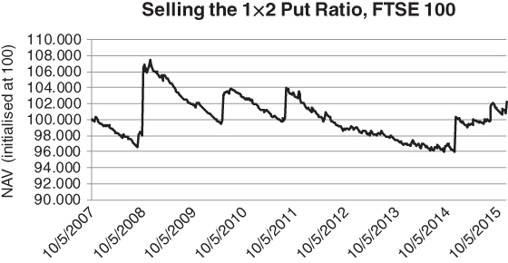Figure 4.12 Short put ratio returns for the FTSE 100, gross of costs

The pattern of returns is roughly the same as for the S&P 500. At this level of gearing, the strategy makes a tiny amount. This is a good result in a portfolio context, as the strategy NAV shoots up during risk events. Recall that a strategy can have a negative expected return yet receive a large allocation in a mean-variance. The beauty of the trade, though, is that a few down weeks are likely to cause a massive shift in the skew. Traders often equate changes in the skew to movements in an oil tanker. It might take a while for the market to react to changes in risk aversion, but once the tanker turns around, there's no stopping it. We will see later in this chapter that risk regimes tend to be persistent over the short term and strongly mean-reverting over longer horizons. The short 1×2 put ratio is something that has been in our arsenal for quite some time. It worked particularly well during the Flash Crash of May 2010, when the put skew steepened dramatically for equity indices and risky currencies.

Our short 1×2 put ratio provides a nice convex payout on the index. It has straddle-type properties. In Figure 4.13, we conduct a non-linear regression of weekly returns for the short 1×2 against weekly S&P index returns. The payout is “non-linear”, as it profits disproportionately from large index moves in either direction. We can see that a quadratic function fits the scatter plot of historical returns reasonably well. This allows us to visualise how the short 1×2 benefits from sharp drops, with no ill effects if the index rises. 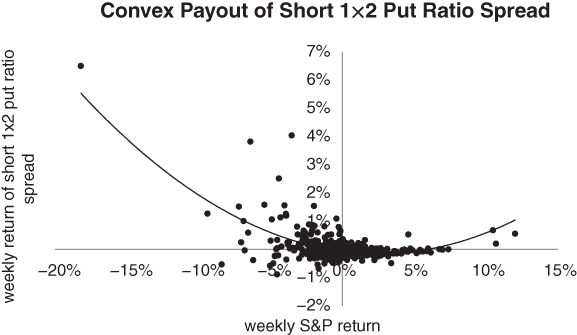Figure 4.13 Convex payout of short 1×2 put ratio spread

At some point, you can get more offensive with the short ratio spread. Suppose, for example, that the S&P 500 has been in an extended sell-off. You believe that a recovery is likely, but realise that the possibility of a complete collapse can't be completely eliminated. The index isn't going to stick in place forever. You can lighten up on the 1×2 by selling a 1×1.5 ratio spread or a straightforward put spread. The 1×1.5 should break even if the index blows through the bottom strike, while generating modest income if the market rallies. If we had to choose one strategy to cover most situations where equity hedging is required, it would probably be the short 1×2 ratio spread. The spread doesn't require perfect timing and can be traded in size. The cost of the structure doesn't go up very much if there is a parallel shift in volatility, which gives us more time to place the trade. However, the distance between the 25 and 10 delta strikes does increase in tandem with volatility. This implies that, if the index drifts down, you will start to fall into a deep well near the 25 strike and may be forced to manage the position aggressively. Managing a position that resembles a long straddle in a high volatility environment can require great skill. The other difficulty with the hedge relates to re-investment risk. Once the S&P put skew expands beyond a certain point, the short 1×2 becomes prohibitively expensive. This means that 2 units of the 10 delta put start increasing in price at a much faster rate than 1 unit of the 25 delta put. If you manage to short the 1×2 in advance of steepening, you profit from relative repricing of the 10 delta put. All is well, as you can take profits on the ratio and roll into a different type of hedge as necessary. But it might be too late to initiate a new 1×2, without having to pay up for the privilege. Once the skew has moved far enough, the structure is too expensive to consider buying.

Some practitioners, who focus on hedging very extreme events, might argue that a 10 delta put is not that far away. It pays out well short of a Black Swan event. Suppose we apply the rule of thumb that the delta of an option is roughly equal to the probability that it will wind up in the money. Then, a 10 delta option has a 10% chance of paying out. On average, you will wind up exercising a static long position more than once a year. This is quite often relative to the perceived frequency of extreme events. We can analyse things from a different angle. The 10 delta strike is only 1.6 or 1.7 standard deviations below the index. This would be a mere drop in the bucket from the standpoint of former Goldman Sachs CFO David Viniar, who claims to have witnessed several 25 standard deviation moves in August 2007. This was in reference to the roughly –27% drawdown suffered by the Goldman Sachs Alpha fund from January to August 2007. The absurdity of such a comment was duly observed by several statisticians, including Dowd (2008). Even a 5 standard deviation move would only have been expected to occur on 1 day since the last woolly mammoth walked the earth (i.e. roughly 10,000 years ago). Mammoths haven't been stomping around for quite some time.

If 10 delta puts offer value, based on the way they reprice during a spike in volatility, 1 delta puts should have even greater potential. These are the Powerball tickets of the hedging world. An investor can make a huge multiple of premium paid in the extreme. We conceptually agree with the idea of buying very low delta options, but will not focus on them in our analysis. It is nearly impossible to assess their effectiveness using conventional statistics. Modelling skew dynamics at the extreme tails of the distribution is fraught with danger. 1 delta put and call prices need to be derived from bid and ask spreads that are typically quite wide apart, as a percentage of the mid-price. The implied volatility skew will be materially different depending on whether you want to buy or sell a “teeny” option. As we move below 1 delta, the situation gets even muddier. The lower the delta, the greater the probability that an option will have a bid price of 0. There might be several options that trade with a 0 bid and a single tick ask, yet these options can't all be worth the same amount. For buy-side investors such as hedge funds, the 1 delta strategy requires a bit of faith. Market makers are reluctant to absorb a large short position in tiny delta options, as this dramatically increases their business risk. This implies that, under most circumstances, you will be forced to pay up for the “teenies”. Back-testing must be performed with great discretion. We are not suggesting that buying large quantities of low delta options is a bad strategy in practice, quite the contrary. If you can truncate the very extreme sell-offs that occur once every 5 to 10 years, your portfolio should compound at a significantly higher rate. However, validating such a strategy is exceedingly difficult and may require a cross-sectional study of extremely rare events.

HEDGING SOVEREIGN BOND RISK

In Chapter 3, we described how to take advantage of large discrepancies between implied and realised volatility. If implied was overpriced, we could sell an option, delta-hedge it and try to lock in the (implied–realised) spread. It follows that the (implied–historical) volatility spread can be used as a valuation metric, a barometer of “fair value”. We can use it as a mechanism for deciding whether options on a given asset are rich or cheap. Some long/short strategies rank individual companies according to this measure. In particular, they sell options on companies where the differential is high and buy options where the reverse is true. Note that we do not know what realised volatility will be over the life of the option and need a rough proxy. The simplest choice is to use some measure of historical volatility as a guide. So long as subsequent realised volatility is not too different from our backward-looking measure, our buy and sell signals should have some information content. Another approach is to forecast volatility, using GARCH or perhaps a homegrown model. However, accurate forecasting is not easy with any model, so we stick with a historical measure for the time being. Let's simplify things by focusing on ATM options. We can then say that, if the spread between ATM implied volatility and historical volatility is persistently small, then ATM options are reasonably fairly priced. By contrast, if the spread is “all over the shop”, it may be that ATM options are subject to cycles of fear and greed beyond what is reflected by spot moves. In Figure 4.14, we can see that ATM Bund options are much more competitively priced than DAX (German equity index) options. We have compared 30-day trailing volatility with implied volatility for a front month ATM put that rolls with 20 days to maturity. 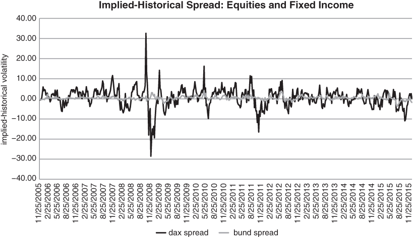Figure 4.14 Spread between implied and historical volatility for Bund futures and the DAX

We acknowledge that, on average, DAX ATM implied volatility is 3 or 4 times higher than Bund implied volatility. This accounts for some of the increased volatility in the (implied–historical) spread. However, the largest DAX (implied–historical) differentials are roughly 10 times higher than the largest Bund ones. This implies that DAX volatility is relatively unstable and that DAX options are more likely to be wildly mispriced from time to time. The same basic relationship holds for the S&P 500 vis á vis the US 10-year Treasury note. Volatility trading opportunities are relatively abundant in US equity indices.

This brings us to the next question. How does the short 1×2 apply to bond futures? We have a squirrely skew to deal with. OTM puts are not always in demand when volatility picks up. After persistent rallies, a call skew tends to emerge. Severe enough sell-offs appear to trigger a put skew, although we have relatively few instances to work with. Figure 4.15 explores the connection between the degree of trending for Bund futures and the shape of the Bund skew. The x-axis tracks the futures price relative to its 100 day moving average. It is a simple trend indicator. The y-axis takes the difference between implied volatility for a 1-month 25 delta call and put, respectively. We can see that, since 2010, there has been a strong positive correlation between the recent trend and the shape of the put skew. The R2 of the regression is roughly 0.10. Whenever Bunds have rallied, a call skew has developed. Whenever they have sold off, puts have gone bid. This is significant, as it suggests that investors are unsure as to whether extreme risks lie to the upside or downside. 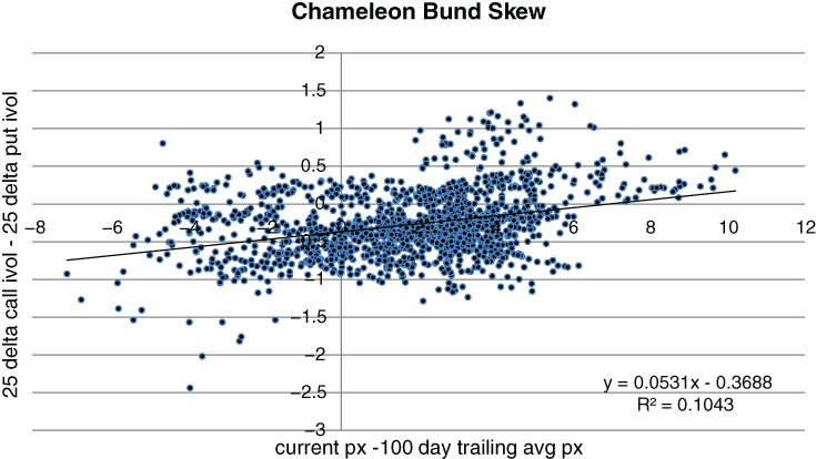Figure 4.15 Bund futures can have a call or put skew, depending on regime

Testing the performance of options structures on bonds is relatively tricky, as they have been in a relentless bull market for decades. This implies that put-buying strategies wouldn't have worked, no matter how clever they might have been. So where can we find enough choppiness to test our theories? We need at least one instance of a major sell-off. Otherwise, we would be inclined to choose a hedge that has relatively low time decay, irrespective of how it might perform during a blow out in yields. “Tail risk” managers are perversely incentivised to do nothing most of the time. So long as nothing too bad happens, they appear to have minimal time decay. Bund futures, while persistently rising, offer the occasional sell off that is useful (though by no means definitive) for our purposes. In Figure 4.16, we graph the performance of a rolling front month strategy in Bund futures, from December 2005 to December 2015. We have chosen our lookback window based on the availability of accurate implied volatility data. 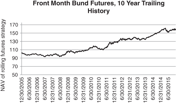Figure 4.16 A relatively long data set with few incidences of sell-offs

There is one sharp sell-off in the data, from April through June 2015. The reader might observe that there was also a decline in Bund futures in the second half of 2010. However, this move was too shallow for a short-term put buying strategy to capitalise on. The one severe drawdown might not seem like much, but it's about all we have to work with. We magnify the chart for 2015 in Figure 4.17, to emphasise the magnitude and severity of the sell-off. 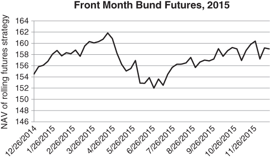Figure 4.17 Close up of price dynamics in 2015

We want to find an efficient structure that would have made a significant amount during the 2015 sell-off. By “efficient”, we mean a structure that doesn't have too much time decay or exposure to the futures roll. A naked Bund futures put would not be very efficient by this standard. If nothing much happened on a given day, your put would lose value based on a combination of theta and forward drift. As we shall see later, bond futures trade in backwardation whenever the yield curve is upward sloping. This pushes the futures away from a downside put strike if the spot (i.e. the cheapest-to-deliver bond) doesn't move.

The consequence here is that you need to overcome term structure effects as well as time decay when buying puts or shorting futures. Our solution is to resurrect the short 1×2 ratio spread as a cost-effective extreme event hedge. If we sell 1 25 delta put and buy 2 10 delta puts against it, our exposure to futures drift will be reduced. We still have to accept that the 10 delta put will burn off quickly at the outset, but are no longer taking the Bund futures head on. In Figure 4.18, we compare the performance of roughly 2 short 1×2 put ratios against 1 long 25 delta put. We have taken some liberties by adjusting leverage on the short 1×2 to match the performance of the long put during the 2015 sell-off. In practice, doubling the size of the short put ratio is sufficient. We have simply matched the performance during a sell-off to highlight the relative time decay in the two structures. 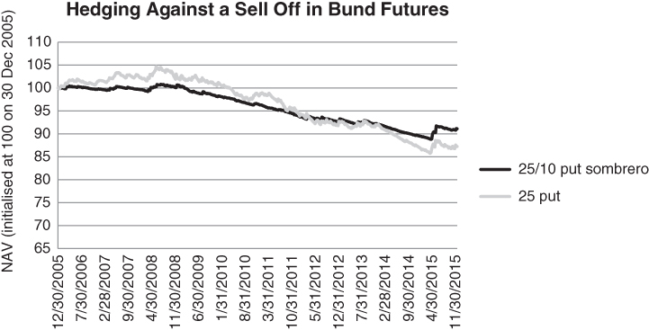Figure 4.18 Relative performance of naked put and “sombrero” for German Bund futures

Neither strategy performs all that well over the entire period. How could they? The futures have been rabbiting away from downside put strikes nearly the entire time. What we can say with some certainty is that both strategies will perform well whenever Bund futures sell-off viciously. If the frequency of 2015-style moves increases, the steady decline in each NAV line may be offset by intermittent spikes. For our purposes, the important point is that the short 1×2 decays more slowly than the outright put, even adjusting for variations in leverage. To be sure, the 25 delta put is relatively responsive to small sell offs. In other words, the grey line is much choppier. However, this should not be a concern if you are focused on extreme event protection.

Up to this point, we have only focused on hedging sharp falls in bond futures. For equity indices, it is usually sufficient to think in terms of downside hedges. Risk is asymmetric, based on aggregate investor positioning. Most institutions have a long equity bias, with large static portfolios of individual stocks, ETFs and indices. Real money accounts, held by sovereign wealth funds, endowments and insurance companies tend to be particularly static. Given their positioning, they are more worried about equity declines rather than “melt ups”. Institutions with interest rate exposure, however, have a wider range of concerns. Bond risk can be two-sided. Bond managers often worry about rising rates, which cause bond prices to fall. Conversely, pension funds worry about a sharp drop in rates. This increases the present value of their liabilities and can render them technically insolvent from an actuarial standpoint. Therefore, it is important to analyse upside call as well as downside put structures. Bonds usually rally during deflationary scares or “flight to quality” events. In a flight to quality scenario, investors are unloading stocks while seeking safe lower duration assets. Cash is king, but investors also have a tendency to stockpile longer duration Treasuries in preparation for an extended downturn. Solvency requirements for banks incentivise the purchase of diversifying assets such as bonds.

We can easily run into difficulty when comparing the historical performance of various upside Bund structures. What was a problem while testing defensive put spreads is still a problem, though in the opposite sense. Nearly every upside trade seems to work in an environment where bonds have been rising and the term structure of futures has been in backwardation. We serve up the 50/25 call spread on the Bund as an example (Figure 4.19). This has been implemented using front month futures options. 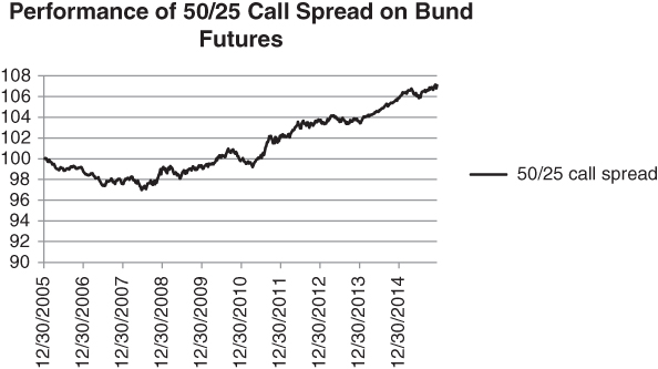Figure 4.19 Historical performance of a call spread buying strategy on German Bund futures

From 2012 on, the graph in Figure 4.19 goes up in a straight line. It's the backtester's dream and the market's bait. Isn't that why people go to quantitative investment conferences, to see hypothetical profits that move inexorably upward? Such steady performance is uncommon for a long options strategy, which has negative time decay by construction. Here, theta in the call spread is offset by a combination of roll down and persistently declining yields. If yields do start to rise and the curve inverts, we should not automatically assume that a call spread will offer protection during a risk event. So long as the term structure is in backwardation, however, the “bleed” of a 50 delta call will be relatively low. You don't lose much from day to day if nothing much happens.

In a steep yield curve environment, call spreads on bond futures do turn out to be elegant hedges, as time decay is partially offset by roll down. We recommend them as “grey swan” hedges against moderate flight to quality events.

SELLING PUT RATIO SPREADS ON THE S&P

It's tricky to say whether very low delta puts are rich or cheap, as we don't and in fact can't know the true probability of extreme events. Our research suggests, however, that 1-month 25 delta puts are expensive with a high degree of confidence. So our core square root hedge relies upon selling 25 delta puts and overbuying 10 delta puts, i.e. we sell a put ratio spread. This structure sells something that is almost certainly expensive to finance something that has a large potential payout. Many hedge funds tend to think in terms of buying the ratio, but presumably focus on options that are closer to at-the-money. Specifically, our analysis revolves around selling a 1×2.5 ratio of 25 and 10 delta puts, so that our initial position is delta-neutral.

THE HYPOTHETICAL IMPLIED DISTRIBUTION

You can get fancy with the implied volatility surface and try to specify the implied distribution of an asset, based on a matrix of option prices. If correct, this distribution would generate the market implied probability of a move of any given size, over any horizon. It would completely characterise the market's collective view on the asset. This idea has been presented by several authors, notably Derman (1999). One way to think of the problem is in the context of binary options. Binaries pay out a fixed amount if the option winds up in-the-money at maturity. Otherwise, they pay nothing. Suppose we have a binary that pays 1 if S(T) lands in the range [S* – delta, S* + delta] and 0 otherwise. Assuming that the drift is 0, the market price of a binary should be equal to the probability of landing between (S* – delta) and (S* + delta) at maturity. In roulette, we face the same sort of payout. We collect a predefined number of chips if the ball lands in the pocket we have chosen and lose our initial bid otherwise. This implies that, if you had a very fine partitioning of strikes, it would be possible to approximate a binary option by a call or put spread whose strikes were very close together. We can label the distance between adjacent strikes as delta_K.

Now we know that, if interest rates are 0, the price of a call spread whose strikes are infinitesimally apart can be approximated by 0.5*delta_K * P(S is between K and delta_K at maturity). Solving for P, we can build a histogram of implied probabilities for the asset. We can then construct relative-value trades by targeting areas where there is a large discrepancy between the options-implied histogram and one constructed from historical data. It's possible to use smoothing techniques to build a continuous implied distribution that is consistent with all prices along the option chain. This circumvents the fact that listed strikes are usually a discrete distance apart.

An accurate implied distribution can give the sell-side a small advantage. In theory, “flow” traders can exploit small irregularities on the implied volatility surface, wherever they might occur. The idea would be to compare the implied distribution of an asset with its historical distribution. A big gap between the two in some regions might suggest a trading opportunity. Note that a flow trader is someone who executes orders on behalf of clients. Flow traders can see order imbalances build up, causing distortions in the skew, and can transact at practically no cost. For buy-side participants, such as asset managers, the implied distribution approach is less useful. Market impact and commissions tend to offset any profits that can be extracted from a minute statistical mispricing across options. As hedgers, we are more concerned with the dynamics of the skew than with a notion of fair value. We want to buy things that will jump in value if there is a risk event, without paying too much for them today. When we back-test options with different deltas, we can check which ones were liveliest during sell-offs. These are the options we want to hold in advance of a sell-off.

You can see that the 10-year trailing performance of the S&P 500, hedged with a short ratio spread, roughly matches that of the index. Buying a 25 or 50 delta put outright is a significant return drag. However, the volatility of the hedged index is 15.41%, compared with 18.25% for the unhedged index. On a risk-adjusted basis, the ratio spread considerably improves a long-only position.

Relative performance in the second half of 2008 might not be clear from the graph. We magnify performance from July to December 2008 below.

OUR FINDINGS SO FAR

Here is a brief synopsis of what we have found. We have focused on options with a month or so to maturity. We have learned that

• risky assets such as equity indices and high yielding currencies have a persistent put skew
• the put skew tends to steepen after volatility picks up
• 25 delta puts seem to be historically overpriced, relative to far out-of-the-money options.

This implies that we want to buy puts further down the skew for low cost protection. Our basic mechanism for taking profits is to roll the strike down if the market shoots toward our long option strikes.

BACK-TESTS: A CAUTIONARY NOTE

In the last section, we argued that whenever you buy an option, you're buying a trading strategy. Your exposure dynamically scales up and down as the underlying asset moves. Given that an option is equivalent to a trading strategy, we back-tested 4-week puts with different deltas to see which ones would have performed best over time. It turns out that, while the 25 delta S&P put looks particularly bad, none of the puts do all that well over time.

So maybe the right idea is to just short puts? Conceptually, this is not a bad idea, as options tend to be overpriced in the absence of an extreme event. On a historical basis, selling puts also looks promising. In Figure 4.20, we short 25 and 50 delta 1-month puts, resetting once a week. The hedging structure from before has been turned on its head. Both the short 25 and 50 delta strategies generate stronger risk-adjusted returns than a static long position in the index. Whereas the S&P 500 only recovers its 2007 peak in 2013, the short put strategies are onside by 2011. 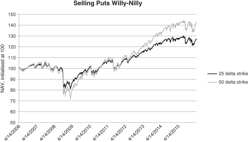Figure 4.20 Superficially, selling puts looks like a fine idea

It seems as though you can achieve an even better return stream by gearing the short 25 put strategy than by selling a single unit of the 50 delta put. We can extrapolate and think of selling 5 10 delta puts rather than 1 50 delta put. However, this sort of reasoning is severely flawed. It invites margin calls and extreme event risk. Gambler's ruin is embedded in this approach, as you are implicitly adding to a losing position on the way down.

When you find a losing strategy, shorting it does not automatically translate to a winning one. At the very least, you need to scale the short strategy correctly. Let's ignore costs for a moment. It's mathematically correct that if you invert a strategy whose average return is negative, the inverted strategy will have a positive average return. However, if the drawdowns are large enough, its compounded return can be negative. A simple example illustrates this point. Imagine a strategy that loses –50% and makes +40% every other month. The returns follow the sequence {–50%, +40%, –50%, +40%, …} and your portfolio descends quickly to 0 with an average monthly return of –5%. If you short this strategy, your return sequence should be an alternating sequence of +50% and –40%. Although the average return is now positive, this sequence also goes to 0, as Figure 4.21 suggests. 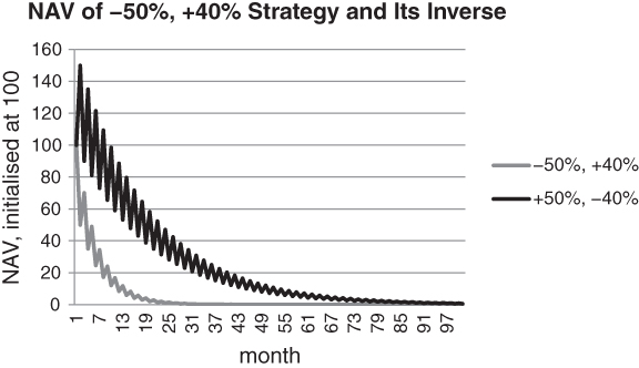Figure 4.21 A strategy and its inverse can both converge to 0 if gearing is too high

Assuming that the {+50%, –40%} ad nauseum sequence is guaranteed, we accept that it is possible to transform it into a winning strategy by reducing leverage. In particular, if you hold 50% cash and invest the remainder in the {+50%, –40%} strategy, your NAV will no longer decay to 0. For any cash balance above 50%, the strategy will be profitable. In Figure 4.22, we assume that 75% of equity is held in cash. 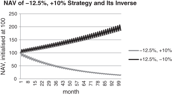Figure 4.22 Inverting a losing strategy does work after dialing down leverage (gross of costs)

For simplicity, we have assumed that the cash return is 0%. Performance is strong, but the essential point is that there is a limit to how much we can do. Readers can delve more deeply into optimal leverage ratios using generalisations of Kelly's Criterion, as in Brown (2011).

Let's drift back to the 1×2 back-test. Some readers might be sceptical of our analysis of the short put ratio. We can't be certain that our back-test is representative of the true return of the hedging strategy. Following do Prado (2013), it might be argued that our verdict suffers from selection bias. The do Prado paper introduces the notion of a “deflated” Sharpe ratio to account for over-fitting and selection bias. Maybe we should refer to it as a manifesto, as it is attempting to overhaul the way systematic strategies are marketed. To a large extent, this is a healthy development. The more configurations you test before arriving at a model, the more you need to penalise the performance of the model back-test. One configuration might be testing a short 1×2 ratio. Another might be testing a short 1×3 ratio, and so on. You also have some flexibility in choosing strikes and the time to maturity of a given structure.

Note that the Sharpe ratio of a strategy is equal to (average strategy return – risk-free rate) / (standard deviation of strategy). After all, from all possible combinations of puts, we have chosen a structure that happened to work fairly well as a hedge in the past. Here, the issue is not one of having over-fit a model. On the contrary, we have not introduced any free parameters into the strategy. But are we guilty of cherry-picking? We take the view that our analysis of the 1×2 is an exercise in hypothesis testing rather than model development. Our initial idea was that many institutions are biased toward hedges that are likely to wind up in the money if there is a sell-off. They tend to over-pay for options that are close to ATM, while ignoring options at the wing. These OTM options can reprice dramatically without ever having intrinsic value. In other words, they don't have to wind up in the money to be profitable. The short 1×2 hedge attempts to exploit this persistent bias. We do not claim that our hedge is optimal in any sense, but have back-tested it simply to show proof of concept. Do Prado and others have argued that it is worth testing a model against simulated data, in an attempt to increase the size of the sample set. However, there are serious difficulties with simulating alternative histories. If you resample individual returns from the past, you lose the precise correlation structure that can lead to trends or other structural tendencies in the data. Even if you resample blocks of data, in an attempt to preserve the relationship between consecutive returns, you might miss the positive feedback loops that drive really large moves. Do Prado is undoubtedly correct when he claims that most back-tests are based on limited amounts of time-varying data. However, the construction of alternative histories is fraught with danger.

We remark that there are glaring examples of selection bias to be found in the investment community. The “stocks for the long run” crowd, referenced in the introduction, claim that equities will nearly always outperform inflation over horizons of 10 years or more. These studies are based on US equity market returns, given the abundance of historical data in the US. This is a reasonable argument, except for one thing. The US is the strongest performing major market over the past 100 years. Success stories are always well documented, in words and numbers. “History is written by the winners”, as the saying goes. Going all the way back to 1900, the five largest capital markets were the US, UK, Germany/Austria, France and Russia. If you had applied modern thinking and allocated to each economy, you would have been wiped out in two of them. You can't restrict yourself to data from the survivors when calculating a risk premium, as ex ante you don't know who they will be.

Before we get carried away with this argument, it is worth pointing out that tabulating data is not necessarily a bad thing. As long as you size positions cautiously, there is no reason to discard information that you have observed. Suppose you were invited to two dinner parties. One of the parties was hosted by someone you had met a few times and gotten along well with. Conversely, you had only spoken briefly with the other host and left with a bitter taste in your mouth. You don't have much to go by, but if you had to make a choice, the first party is obviously preferable. While mean reversion effects need to be taken into account with financial data, the basic principle is the same. There is every reason to use the available data, so long as you do not place too much confidence in what you have found.

A SHORT DIGRESSION: DELTA-NEUTRAL OR COMFORTABLY BALANCED?

You can construct positions that are delta-neutral but highly imbalanced. If you short a large number of straddles that expire tomorrow, you are initially delta-neutral, but your position is hanging on a knife edge. The profit from the trade will be highly dependent on your ability to delta-hedge at the right moments. Any trade that induces severe physical symptoms is by definition imbalanced. For winning trades, it is tempting to think, if only the position had been larger. But if you had done more, you would have needed to tighten your risk controls to the point where you might not have made any more money. This is a reasonable, if heuristic, argument for sizing open-ended strategies conservatively. We are doing this for your health.

THE 665 PUT

We conduct a small and hopefully amusing Gedanken experiment in this section. However, the experiment does have important consequences. Namely, it shows how margin constraints need to be factored into any strategy that incorporates leverage. The year is 2005 and you have a vision. You divine that, however tumultuous markets may become, the S&P will never close below 665. 665 is a rock solid floor. Note that we did not choose 666 as the floor because S&P index option strikes appear in multiples of 5. Nostradamus will not factor in our experiment. The rest of the future is not revealed to you. As you sit mulling things over, you realise that you have a strategy that can't lose. All you need to do is sell a 1-month 665 put, wait until expiration, and repeat. If your vision is true, the put will always expire worthless. The worst-case scenario is that you won't collect much premium when the S&P is well above the strike. To an extent, you can adjust for this by maintaining a relatively constant margin-to-equity ratio over time. In master of the universe mode, you aggressively trade according to the following rule in your brokerage account.

• Once a quarter, you decide how many 3-month 665 puts you are going to sell, by setting your margin to equity ratio at 50%. In other words, you have 50% cash to support your positions.
• At the end of the quarter, you cash out any gains from the quarter. These are no longer usable as margin as they have been deployed elsewhere.
• You then sell the appropriate number of 665 puts, with end-of-quarter expiration. This assures that no rebalancing will take place along the way.

Now, let's wind the clock forward to 2015. The thought experiment is about to take a dramatic turn. You sit comfortably in a plush chair bought with the gains you expect to realise now. After all, expectation is a form of wealth. However, your deputy is nowhere to be found. Nonetheless, it is time to review your statements and congratulate yourself on the cumulative result. Your vision was correct, as the intraday low for the S&P was 666 on March 6, 2009. All must be well. As it turns out, there are no statements from 2010 to 2014. You defaulted, in the sense that your account was liquidated by the broker in March 2009. How can this be? You had a sure-fire trading strategy. You gave yourself some wiggle room by leaving 50% of the account in cash, to cover mark-to-market losses. No dice. As Figure 4.23 suggests, the problem was the way you sized positions. Neither your broker not the exchange could give you credit for perfect foresight. 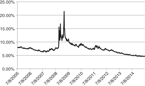Figure 4.23 Estimated margin requirements for short 665 put

Figure 4.23 estimates the exchange margin requirements for 1 short S&P 665 put. While your broker may require more margin, this is a lower bound on what you need to post. If you short a put listed at the CBOE, the initial margin required is equal to the (put price) + 0.15 * (put strike). In the graph, we have simply converted the margin required into a percentage of the index level. Recall the way we sized the strategy. Sizing is a bit contrived, but instructive. We agree to harvest gains from the previous quarter, to the point where there is a 50% cash buffer at the beginning of a new quarter. The strategy gets knocked out if the margin requirement ever doubles from its initial level at the beginning of the quarter. Can we please remind the reader again that back-tests don't have emotions? It's not simply a question of leverage constraints in the example above. Once you are in trouble, the high probability of a recovery stipulated by your model is not enough to rely upon.

IMPLICATIONS OF THE SQUARE ROOT STRATEGY

We have analysed the short 1×2 put ratio in some detail, as a low-cost hedge against a severe drawdown. Short 1×2 call ratios also have a function, e.g. as an extreme inflation hedge. We might sell a call ratio on a commodity index if a bubble seemed to be developing, i.e. if the move seemed overdone, but might go “parabolic” before reversing. If we wanted to hedge both extremes while harvesting some premium, we might wind up with a 2-sided ratio spread, such as the one following.

Figure 4.24 can be viewed as a blueprint for investing and risk taking in general. Our internal code name for the strategy used to be “sombrero”, based on the payout profile at maturity. (A “Stockton hat” would have been a more accurate description, but we are no hat experts.) This sent brokers scrambling to the internet when we placed an order, to no effect. They typically had no idea what we were talking about and were afraid to ask. In reality, a sombrero is just a 2-sided short ratio spread. The code name was a concise and amusing way to describe it. 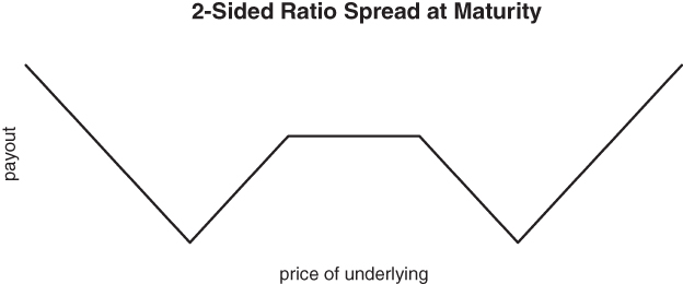Figure 4.24 2-sided ratio spread, payout at maturity

Many, if not most, investment strategies rely on capturing a risk premium of some sort. These include deep value/distressed investing, FX carry, buying the target stock in a potential merger, selling volatility among others. In each case, you are collecting a return for bearing risk that some segment of the investment community can't tolerate. This is all well and good, but if your strategy involves any leverage, it can get wiped out during an extreme event. So it is absolutely vital to include low-cost, low-delta options as part of a risk premium harvesting strategy. Once you add OTM hedges, your composite position resembles a condor. If you buy the wings more aggressively, you wind up with a short 2-sided ratio spread in spirit. Are these far OTM options rich or cheap? At some level, it really doesn't matter. So long as your hedge-adjusted carry is large enough, the “teeny” option hedges are simply the cost of doing business. Over-buying options at the extreme gives you the opportunity to add to your risky trades as they become more attractive or take some profits at the wings while maintaining a hedged book.

FUTURES VS SPOT

Suppose we take the view that crude oil is about to go up. We want to profit from an increase in price, but don't have the infrastructure to receive, store and deliver physical oil. A natural alternative is to buy crude oil futures. The front-month futures should move roughly in tandem with spot oil prices. By “front-month”, we mean the live contract that has the least time to maturity, yet significant open interest. In order to maintain our long position over time, we need to “roll” the contract before it expires. Rolling involves selling front-month and buying back-month futures to re-establish the position. The back month is the next active futures contract along the term structure.

Now suppose that the term structure is “in contango” at the short end of the curve. This means that front-month futures are trading at a discount to the back month. If we want to roll our long position, we need to sell low and buy high. More precisely, we have to pay (front month price–back month price) / (front month price) in percentage terms to maintain our long position. This is our roll yield and in this case is negative. The implication is that roll will materially impact our returns if we wish to hold a position for a long time. As we will see later, cumulative roll yield can have a larger impact on your overall return than changes in the spot price! When the short end of the term structure is in severe contango, it is tempting to think about buying long-dated futures. This offers two advantages. The long end tends to be relatively flat, reducing roll down from one month to the next. In addition, you don't have to roll quite so often. The trouble with this strategy is that long-dated futures can be relatively illiquid and more importantly, they might not respond enough to a jump in the spot price. When there is a supply shock in a market such as oil, front month futures tend to jump. The market prices some mean-reversion further along the curve and the effects can be muted there.

A DRAMATIC EXAMPLE

We start with an extreme case, to highlight the potential impact of roll down. Our opening gambit involves trading the yield curve, which is structurally similar to the futures term structure. Imagine that we stumbled upon a yield curve in the shape of a step function, as in Figure 4.25. 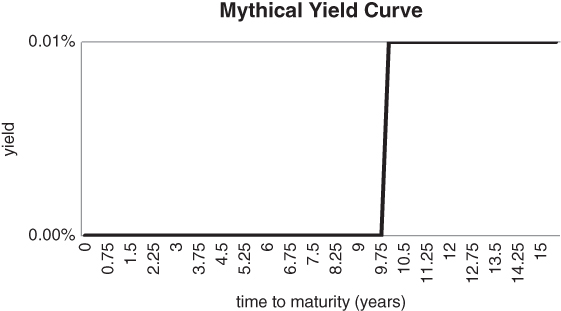Figure 4.25 Mythical yield curve: roll down, rather than absolute yield, can generate attractive returns

Yields are uniformly low, in absolute terms. From a long horizon asset allocation standpoint, bonds look like a terrible buy. If you hold any bond along the curve to maturity, your annualised return will be less than 1 basis point, or 0.01%. This is unlikely to excite anyone unless the underlying economy slips into a severe deflationary spiral. From a trading standpoint, however, there is a fantastic buying opportunity embedded in the curve. It's unimportant that the absolute level of yields is low. All you need to do is buy a 10-year 0 coupon bond. The yield curve is infinitely steep at the 10-year point. Assuming no change in the curve overnight and a par value of 100, the bond reprices from 100exp(–0.000110) = 99.90 to 100 in one day. Assuming 252 trading days per year, this corresponds to an annualised return of 29%! The alchemy of a steep yield curve allows you to convert low yields into high returns.

The same logic applies to forward curves, though with opposite sign. Note that bond prices move inversely to yields, so that a steep yield curve favours a bond buying strategy. If you buy futures on a commodity such as heating oil, an inverted forward curve creates positive carry. When the term structure is downward sloping, it is said to be in backwardation. Front-month futures are trading at a premium to deferred contracts. The mechanics of maintaining a long position when the futures term structure is in backwardation are illustrated in Figure 4.26. 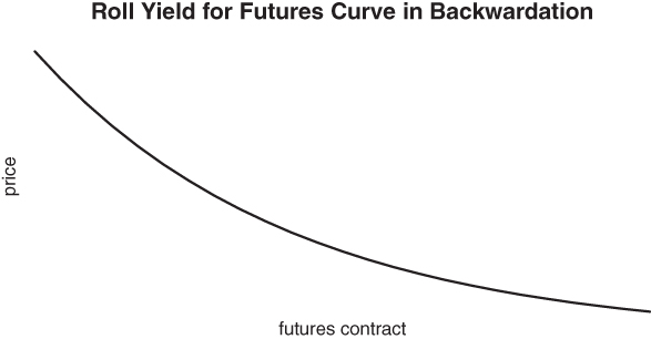Figure 4.26 Maintaining a continuous long position in a market where the term structure is in backwardation

While our “mythical” yield curve strategy relied upon unwinding a 10-year 0 coupon bond every day, futures are generally rolled once per expiration cycle. Rolling a long position requires selling the front month while re-establishing a long position in the back (i.e. second actively traded) month. So long as the curve remains in backwardation, you can keep selling the front month at a higher price than you buy the back month. This generates a return equal to (front month price–back month price) / (front month price) each time the contract is rolled. Sovereign yield curves tend to be upward sloping more often than not, as investors typically demand compensation for bearing duration risk. This suggests that the roll yield for bond futures contracts should typically be positive.

It is instructive to quantify the long-term impact of roll yield on investor returns. In the next section, we will show that roll yield dominates spot price movements for most physical commodities over long time horizons.

A CROSS-SECTIONAL STUDY

Till (2006) provides concrete evidence that returns from a rolling futures contract on a commodity are distinctly different from returns on the spot commodity itself. This can have a bearing on our decision to take a directional bet in the futures markets. If the inherent roll yield is negative, you need to have high conviction or a short target holding period to justify buying the futures.

Suppose you take a bullish long-term view on gold, on the assumption that central banks will engage in the competitive devaluation of their currencies. You can't buy physical gold, as you neither have a place to store it nor a mechanism for receiving and delivering it. So you wind up buying gold futures and rolling every so often. Also suppose that the futures term structure is in contango, implying that long-maturity futures trade at a premium to short-dated ones.

In order to maintain the gold position, you have to roll the futures, typically as open interest moves from one contract to the next. If the curve remains in contango, rolling is persistently costly. You repeatedly have to sell the front month futures at a lower price than you are buying the back month. In other words, you are selling low and buying high over and over again, so your carry is negative. So when you trade gold futures, you are not really trading physical gold, but a combination of the spot commodity and its cost of carry. This applies uniformly to all futures contracts where the term structure is not completely flat.

Various authors have studied the relationship between physical commodity returns and returns from a rolling futures strategy on the commodity. Over long horizons, it turns out that the shape of the term structure is the decisive factor. Moves in the underlying asset are overwhelmed by roll yield. Figure 4.27 updates the analysis of Till (2006), with minor modifications. We cover 10 of the most actively traded physical commodities, using data from 1995 to 2015. The x-axis gives the average level of backwardation for each commodity. More specifically, if the price of the front and deferred month forwards are F1 and F2, respectively, we calculate (F1 – F2)/F1 for each commodity. We then average (F1 – F2)/F1 over the entire period. 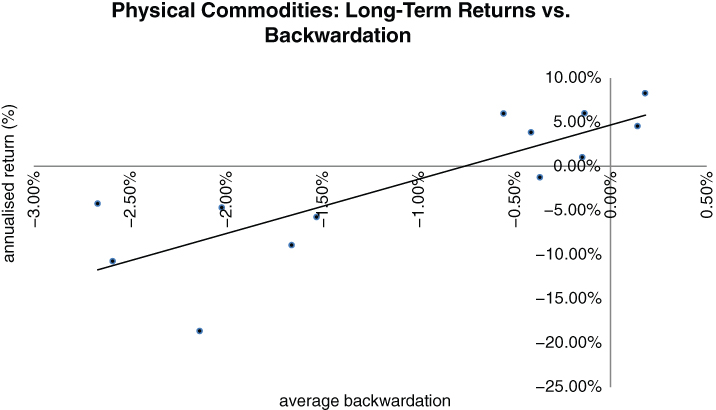Figure 4.27 Impact of futures term structure on long-term returns for various physical commodities

We can draw several meaningful conclusions from Figure 4.27. Most of the dots are to the left of the y-axis. This implies that commodity term structures tend to be in contango. Roughly speaking, contango is more common than backwardation. Secondly, the regression line is strongly upward sloping, with an R2 around 0.65. The persistently backwardated commodities, namely soybeans and heating oil, have the best long-term rolling futures returns. Commodities in trade in contango in the absence of a supply shock, such as natural gas, have very negative annualised returns. One might argue that there are only 10 points in the scatter plot, implying that the regression is based on a thin data set. We would argue, however, that by averaging the quantity (F1 – F2)/F1 over 20 years of weekly data, each dot is a solid one. The points on the graph are not very noisy.

It should now be apparent that there is a strong relationship between the average shape of the term structure in a given market and realised futures returns. Accordingly, it seems advantageous to roll long positions in markets that are typically in backwardation and to roll short positions in markets that are in contango. Both strategies generate positive carry over the long haul. Bond futures, stock index futures in a low interest rate, high dividend environment and the odd commodity (e.g. heating oil) are good candidates for a rolling long strategy.

A cautionary note is in order. It's one thing to keep buying a contract that is regularly in backwardation for a definable structural reason. That straightforward strategy seems to work, at least over a long enough horizon. What doesn't work is an attempt to jump in and capture roll yield when a curve that is normally in contango suddenly goes into backwardation. For example, natural gas futures may switch into backwardation after a supply shock. Short-term prices rise more than long-term ones, as investors assume that the current shortage will eventually be remedied. However, the futures curve at this point can be very unstable. When you buy front month futures on the assumption that it will be possible to roll at a lower price in the future, you are assuming that the shape of the term structure will not change much over time. This assumption can be a disastrous one after a supply shock. Spot gas prices can decline very quickly, forcing the term structure back into contango. In this case, your implicit curve trade (long front month and short back month futures) will go strongly against you.

In the next graph, we explore the relationship between the level of backwardation of natural gas futures and its 4-week forward return. The graph is based on historical futures data from 1995 to 2015, at weekly intervals. Let's denote the front month futures price by F1 and the deferred month price by F2. The degree of backwardation relative to the front month contract is given by (F1 – F2)/F1. When F2 > F1, the term structure is upward sloping, or in “contango”. When F2 < F1, it's in backwardation. We can now compare forward returns over some horizon to the degree of backwardation in the term structure. The results are summarised in Figure 4.28, assuming that we calculate forward returns over a rolling 4-week interval. 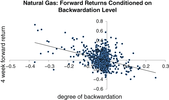Figure 4.28 Prospective natural gas futures returns actually drop when the curve goes into backwardation

Buying natural gas after the curve has inverted is a losing strategy. It is true that long-term performance is primarily driven by an aggregation of negative returns when the curve is mildly in contango. This is the scenario that occurs most frequently. However, the best individual returns occur when the gas curve is steep and the worst returns when it is inverted. It may be that the severe contango returns are based on an implicit value play. The denominator F1 in (F1 – F2)/F1 is relatively low. Conversely, the snap back after curve inversions can be vicious.

How do things stack up on a cross-sectional basis? The results are similar and given in Figure 4.29. We have repeated the natural gas regression for a larger collection of physical commodities. The historical look-back window is 20 years. 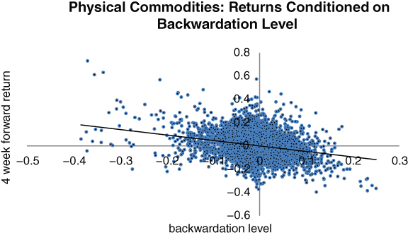Figure 4.29 Cross-sectional dependence of returns on level of backwardation

The results are broadly similar. Most of the points are to the left of the y-axis, suggesting that storage costs and other considerations usually force the term structure into contango. Episodic moves into backwardation should be sold, as the odds favour normalisation of the curve. If roll yield is to be exploited over the long term, it needs to be reliable. Buying front month futures after a supply shock just doesn't seem right. Dedicated commodity traders are always on the lookout for term structures that have gone into backwardation. They usually try and squash the spread by selling front month futures and hedging further along the curve. Anecdotally, these traders tend to make money most of the time. It is debatable whether they take extreme event risk to collect if the curve flattens, but this is beside the point. You are unlikely to make consistent profits by taking a long position in front month futures after a risk event without exceptional timing.

What you really need is a market that is persistently in backwardation. So long as the yield curve is upward sloping, Treasury bond futures are an excellent choice. From 1982 to 2015, the US 10-year yield has been higher than the 3-month T bill rate roughly 90% of the time. Given an upward sloping yield curve, 10-year note futures have to trade at a discount to the cash bond. Note that we have glossed over several technical details here. For example, there is a basket of notes that can be delivered into the futures contract and they may have much shorter durations than 10 years. However, the rough argument goes as follows. If the futures traded at par to the cheapest-to-deliver cash bond, you could make a guaranteed profit by selling the futures and borrowing money to buy the deliverable bond. Then, you would be flat at maturity, having collected an annualised return of (deliverable bond yield – T bill yield), which is greater than 0. As you go further out the curve, the futures will generally decline in price. The same arbitrage argument applies, with a cheaper cash bond and a greater interest rate differential between the bond yield and the cost of borrow. In the absence of conversion factors, we are applying a larger discount to a cheaper bond. Hence, given an upward sloping yield curve, bond futures should trade in backwardation.

THE “New” VIX: MODEL-INDEPENDENT, THOUGH NOT PARTICULARLY INTUITIVE

At this point, we move into a discussion of what the VIX is actually measuring. From 1990 to 2002, the VIX was calculated in a relatively simple way. The calculation relied upon taking the three closest to ATM options in the front two months, then applying Black–Scholes and doing some averaging. In particular, the three closest strikes would be averaged according to their distance from the ATM strike. The front two months would then be averaged, based on their distance from a constant 30-day-to-maturity window. Note that the original VIX calculation was derived from S&P 100 options, while the new one focuses on the S&P 500.

At some point, model-dependent quantities became verboten, no longer tradable according to the regulators. We find this amusing, since the regulators have no hesitation in accepting model-dependent risk calculations based on Value-at-Risk or other methodologies. The current VIX is based upon the pricing formula for a variance swap, as in Carr (1998). A variance swap is a contract that pays out based on the difference between realised variance and the swap “strike”. The strike is based on the market's expectation of future realised variance. It turns out that the variance swap strike can be priced directly from a weighted average of market call and put prices, without reference to Black–Scholes or any other pricing formula. The contribution of an OTM call or put with strike K is proportional to 1/K2. This implies that deep OTM puts (i.e. where K is small) can have a large impact on the price of a variance swap if their prices are not too small. As the prices of calls and puts rise, expected variance goes up as well. The new VIX is just the square root of the variance swap strike.

The updated VIX formula does have some advantages over the original one. In particular, it incorporates all available strikes, which gives a slightly more skew-dependent view of the level of risk aversion in the market. Variance swaps also have a fairly pure design, as pricing does not require any assumptions about the distribution of the underlying asset. It has been shown, as in Hiatt (2007), that the new formula tracks the old one quite accurately. The downside is that the average Joe doesn't understand the intricacies of the new calculation. Tradable quantities probably should not rely upon complicated mathematics. It is not Joe's fault if he is afraid that the more complicated formula might start to wildly diverge in the future, as the extremities of the put skew become distorted.

THE SPOT VIX: OASIS OR MIRAGE?

In theory, the VIX can be an attractive hedge for a number of reasons. The correlation between the VIX and the underlying S&P 500 index (SPX) has historically been very high and negative, in excess of –80% using daily observations. Although mean-reverting, the VIX tends to have more than 5 times the volatility of the SPX. It is far more likely that the VIX will double than that the SPX will drop by –50% over a short horizon. This suggests that a relatively small position can go a long way. Unlike an option, the spot VIX does not have explicit time decay.

In the introduction, we mentioned that if you could predict crises with perfect accuracy, hedging would be either trivial or unnecessary. The same line of thinking applies to the spot VIX. If you could buy the spot VIX, hedging a portfolio of risky assets would generally be quite easy. Unfortunately, this is a giant “if”. You could hold a static long position in the spot VIX against your portfolio of equities or credit. There might be ways to optimise things further, but this would be an excellent starting point. Note that the spot VIX is the number quoted by the media. It has two characteristics that constitute an ideal hedge, i.e. persistently negative correlation to the S&P 500, with no time decay or negative carry. In Figure 4.30, we track the performance of an unlevered portfolio consisting of a 90% position in the S&P 500 and 10% in the spot VIX. A dash of the VIX does wonders for your overall portfolio. 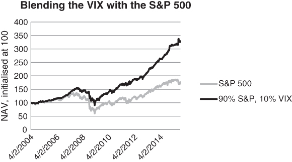Figure 4.30 Impact of 10% spot VIX allocation to S&P index returns

The results are astonishing. The blended portfolio has roughly double the compounded return of the index. The NAV (net asset value) virtually moves in a straight line from 2009 to the present. This seems too good to be true. We appear to have stumbled upon a very basic strategy that has enormous alpha. Does the market really give things away so easily? In the case of the VIX, the answer turns out to be a resounding no. When we try to implement a VIX buying strategy, it immediately becomes clear that the returns in the above chart can't be replicated. It is not possible to buy the VIX directly. In practical terms, the VIX doesn't exist; the quoted number is virtually useless for a buy-side investor. It is true that the VIX calculation is based on a weighted average of prices for listed S&P options. However, you would have to constantly rebalance your replicating portfolio as the index moved, to ensure that all of your options were out of the money. You would also have to pay through the bid ask spread for deep OTM puts that can have a meaningful impact on the index. The replicating portfolio would consist of hundreds of OTM calls and puts, creating an awful mess. Rebalancing would be prohibitively expensive from a buy-side perspective.

futures offer a direct way to express a view on S&P volatility over short horizons. They have been listed at the Chicago Board Options Exchange, or “CBOE”, since 2004. At maturity, VIX futures have to converge to the spot VIX, so there is a close functional relationship between the two. It is tempting to conclude that you can leave precise replication to the banks and just buy the futures. The impracticality of this approach becomes apparent when we replace the spot VIX with a rolling position in VIX futures in the blended 90%, 10% portfolio above as shown in Figure 4.31. 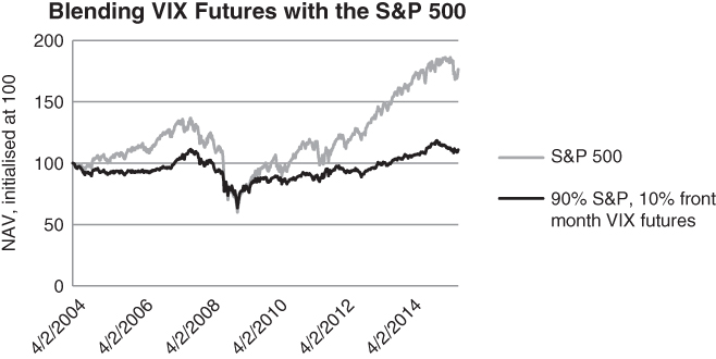Figure 4.31 Impact of adding VIX futures to static long S&P 500 position

While the spot VIX materially improves risk-adjusted returns, VIX futures dramatically reduce performance. Buying and rolling VIX futures is an outrageously expensive way to protect against disaster. The difference in performance is astounding and at first sight, surprising. How can this be so? We have simply replaced the spot VIX with the forward VIX in our calculation. The trouble is that the VIX futures term structure tends to be in severe contango most of the time. The VIX is not a deliverable commodity and the term structure of VIX futures reflects excess institutional demand for hedging. The structural imbalances driving the VIX futures curve have created trading opportunities that have attracted the attention of yield curve traders and other “arbitrageurs”.

We have reached a critical juncture. Why not apply the VIX formula and simply try to replicate it? If replicating an S&P index put with the underlying is dangerous in the presence of jumps, VIX replication is practically impossible for most buy-side investors. As the saying goes, you can't buy the spot VIX any more than you can buy a sunny day. Hedging with volatility turns out to be a challenge after all. Reasoning from the VIX formula, you would have to own every OTM put and call with open interest and rebalance whenever the ATM strike moved. On average, you would have to rebalance several times a day, as the following order of magnitude argument suggests. Suppose the S&P 500 is trading at 2000. S&P options strikes are typically 5 points apart or 0.25% of the index. In quiet market conditions, a 1 standard deviation 1-day move is roughly 1%, implying that you would have to buy and sell large quantities of options several times a day. The costs would rack up, given that you would also have to rebalance daily to maintain a constant 30 maturity profile.

To understand the impact of negative roll yield, we need look no further than the data. In Figure 4.32, we track the front-month VIX futures premium over the spot VIX, as a function of time. While the spread between futures and spot has been quite volatile, we can see that the average futures premium has been very high, at around 6%. The difference between the front month futures price and the spot is commonly referred to as the basis. 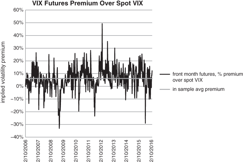Figure 4.32 Historical VIX futures premium over spot VIX

The traditional basis is of concern if we hold to maturity. For perpetually rolling strategies, we are more worried about the spread between front and second month VIX futures. This will determine the cost of maintaining a long position. In Figure 4.33, we track the average level of contango at the short end of the VIX term structure. This is a different convention from the one used by Till and Eagleeye (2003). We are now thinking of the cost of maintaining a long futures position, rather than the risk premium collected for contracts that are in backwardation. Specifically, we trace the evolution of the quantity (second month futures price–front month futures price) / (front month futures price) from 2006 to early 2016. 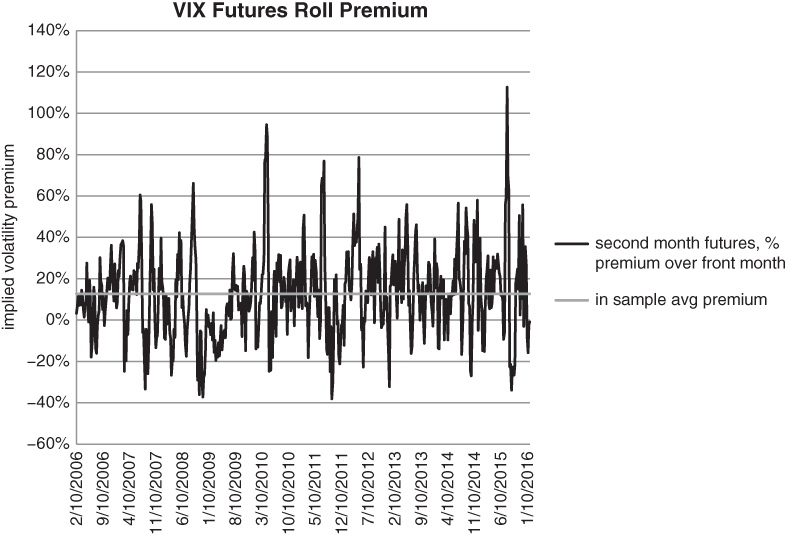Figure 4.33 Front month VIX futures premium over second month, historical perspective

The straight grey line is an in-sample average over the entire period, with dire implications. We would have had to buy roughly 10% fewer contracts in the back month each time we rolled, assuming we didn't add cash to the position. This suggests that our volatility hedge would have simultaneously lost money and withered away over time. The implication is that we do not want to take the VIX head on. Maintaining a long volatility position by mechanically rolling VIX futures is simply too expensive. One thought is to buy OTM call options on the spot VIX, on the assumption that roll down exposure is relatively indirect. The trouble with this idea is that, although the calls settle based on the spot VIX at expiration, they trade with reference to the VIX futures. Your instantaneous roll down is equal to (call delta) * (roll yield of equivalent duration futures). So you still have fractional exposure to roll down, which is compounded by time decay in the call.

Whether in futures or options form, the VIX is not a buy and hold instrument. You have to finesse or time it in some way. But if you could market time VIX futures or options, why would you need them in the first place? You could simply exploit the high structural correlation between the VIX and S&P 500 by selling an appropriate number of S&P futures whenever you had a VIX buy signal. This would give you similar (though perhaps less explosive) exposure, while eliminating roll down.

Structural challenges are one of the things that make investing interesting and perhaps we should view things differently. A potential solution is to revisit the short S&P ratio spread idea, with a twist. Rather than trading a ratio spread, you can sell VIX futures while overbuying OTM VIX calls. Selling a call ratio spread turns out to be sub-optimal, as 10 delta VIX calls do not offer value to the extent that 10 delta S&P puts do. Before investigating the short futures, long calls strategy, we need to analyse the peculiar properties of VIX options. This is the subject of the next section.

MIGRATING TO VIX OPTIONS

This section culminates with a strategy that provides a convex payout on the VIX, at relatively low cost. The strategy turns out to be particularly useful during risk off regimes, when standard hedges are invariably overpriced. We first need to discuss some of the intricacies of VIX options, before constructing our hedge.

We have observed that, while VIX options settle with reference to the spot VIX, their price depends upon a VIX futures contract with the appropriate maturity. For example, if you bought a September VIX call, you would plug the September futures price (rather than the spot VIX) into Black–Scholes to value the call. This is logical. September VIX futures give the market's best estimate as to where the spot VIX will land at September expiry. What makes things complicated is that VIX futures do not depend upon the spot in a purely deterministic way. They are not priced according to a standard cash and carry formula. Indeed, there is no simple formula that allows you to price the VIX forward curve as a function of prevailing interest rates and the spot. Rather, they reflect supply and demand dynamics for S&P options and the futures themselves over different time horizons. In this respect, they are qualitatively different from physical commodity futures.

This suggests that long-dated calls may not appreciate as much as one might expect during a risk event. If the spot VIX jumps from 20 to 50, we should not expect that a 3-month 50 strike call will be at the money. The futures term structure prices in a degree of mean reversion and it may well be that the 3-month futures are closer to 20 than 50. As a result, we can't rely on long-dated VIX calls to hedge against intermittent, short-term risk events. They will probably not be responsive enough.

An obvious alternative is to focus on front-month options. In principle, short-dated VIX calls can be powerful extreme event hedges. However, you face multiple headwinds when buying VIX calls that are close to maturity. Roll down tends to be highest at the short end of the term structure. As a result, you face the double whammy of high time decay and severe roll down. However, there are compensating factors. At the very least, short-dated OTM VIX calls are lively. Suppose you buy 1-month S&P 500 put. If the index rises +10% over the course of a few weeks and then suddenly drops –10%, the put will usually lose money. Time will have passed without a net change in the spot. Close to expiration, the put delta will have fizzled away. However, a 1-month VIX call will probably make a sizeable return as the VIX will likely be much higher than it was at the beginning of the period. Out-of-the-money strikes remain in play late into the expiration cycle. Over a modest horizon, the VIX is much more likely to double than the S&P is likely to decline by –50%. Hence, VIX calls are far more likely to jump in the money than S&P puts, especially close to maturity.

Structural issues are also at play. The VIX options market is perverse in the sense that it almost encourages VIX futures to overshoot fair value. In particular, the open interest in VIX options exceeds VIX futures open interest. If the majority of speculators were short OTM VIX calls, there would not be enough inventory to delta hedge them during a risk event. When we also consider the intrinsic jumpiness of the VIX, replicating a short call seems extremely dangerous. If a large enough number of investors tried to hedge a short call with futures, there might be enough buying pressure to drive very high strike short-dated calls into the money.

A nice feature of VIX calls is that they become more potent close to expiration. In this way, they resemble the put and call butterflies we discussed earlier. We know that any futures contract has to converge to the spot at expiration and VIX futures are no different. The interesting thing here is that long-dated VIX futures are not nearly as volatile as the spot VIX. The market prices a certain amount of mean reversion into the futures. This suggests that the futures should become increasingly volatile as the time to maturity shrinks. We show this in the sparse Figure 4.34. We consider the front four VIX futures contracts in the graph. These have expirations that are one month apart. Next we calculate the rolling 30-day standard deviation of each contract as well as the VIX. We then graph the ratio of each standard deviation to the standard deviation of the VIX. The futures roll is transacted one week before maturity. 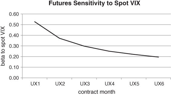Figure 4.34 Front month VIX futures are relatively responsive to changes in the spot VIX

The front month futures are highly responsive, with a beta over 0.5 to the spot VIX. They jump around more actively than the other ones. This implies that an OTM VIX call should be nice and lively close to expiration. High strikes are more reachable late in the cycle. So long as VIX implied volatility is not egregiously priced close to expiration, weekly options can again offer tremendous potential payouts.

Before we get carried away with the idea of buying boat loads of low delta VIX calls, we need to keep one thing in mind. We don't derive the same benefit from the VIX call skew as from the S&P put skew. We have seen how the S&P put skew can steepen during a crisis. This gives an extra price kicker to an OTM put on the S&P. While ATM volatility does tend to spike at these moments, the call skew may flatten or even decline at the wing. The market may price some mean reversion at the far reaches of the VIX call skew. This strategy creates a convex payout on the VIX. It is well known that VIX futures generally trade in severe contango, which implies that a rolling long position has overwhelming negative carry. Front-month VIX futures have traded at an average discount of roughly 6% to the back (second) month. This compounds aggressively over time. The VXX (a US ETF that implements a rolling position in front month VIX futures) has lost –99.72% since its January 2009 launch and has required several 4:1 reverse splits to trade at a reasonable level!

Let's combine this information: front-month VIX futures usually trade at an unacceptable premium to the spot, and roll down affects a VIX call at a declining rate as the futures roll toward the spot. Can we build a strategy from these observations? One solution is to sell VIX futures while overbuying VIX calls. This allows you to capture roll down on a 1:1 basis from the futures. Meanwhile, the exposure of the calls to roll down diminishes over time if the spot doesn't move. Conversely, if the VIX goes heroically bid, you quickly go from a short to a long delta-adjusted position. This suggests that the strategy should produce a convex payout on the VIX. The data bears this out.

Let's take a concrete example. In the chart below, we compare weekly returns for a long position in the VXX with a short position in the VXX coupled with 1.5 long 25 delta calls. If volatility either drops or rises a lot, the short VXX, long 1.5 VXX call strategy benefits dramatically. The payout is distinctly “straddle-like”, without your having to pay a premium on both sides. While the intercept of the quadratic regression is negative, the strategy actually produces positive alpha relative to a long position. Most points in the scatter plot are to the left of the y-axis, some far to the left, which ensures that the VXX compounds in a horrible way.

The relative performance of our hedge against a long VXX position is shown below. Note that both strategies lose money in isolation, but our hedge outperforms quite dramatically. Also observe that the y-axis is in log units, which dampens the observed moves in our hedge but allows us to compare the relative roll down in the two approaches.

For every VIX futures contract that we short, we need to buy 15 50 delta calls to construct a position that is initially delta-neutral. The ratio is 15:1. Note that we buy 15 rather than 1.5 VIX calls as the futures contract multiplier is 1,000, whereas the options multiplier is 100. A short futures/long call strategy is conceptually similar to the short 1×2 put ratio on the S&P 500 that we discussed earlier. If volatility spikes, delta becomes strongly positive and the structure offers significant protection. Conversely, as volatility declines, the call deltas decrease. The structure then has net negative delta, i.e. is locally short volatility. This implies that your delta-adjusted exposure to roll yield is positive. You benefit from a term structure in contango at an ever-increasing rate. Relative to a rolling long position in VIX futures, the variable delta of the structure generates alpha. Figure 4.35 relies upon weekly data from 2006 to 2015 and suggests that the short futures/long call strategy is generally superior to a rolling futures benchmark. 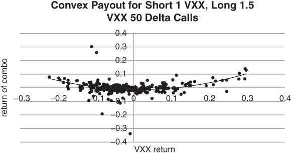Figure 4.35 Convex payout of strategy where VXX calls are overbought

The weekly alpha in the trade is 35 basis points, corresponding to roughly +20% annualised outperformance! While the strategy still loses money in the absence of market timing, it is not consistently hampered by negative roll yield.

The scatter plot suggests that the payout function is mildly convex relative to a rolling VIX futures strategy. This can be appealing if the VIX has recently spiked. You reason that risk aversion levels are not going to stay put. The market is at an unstable equilibrium, similar to a pendulum that is hanging upside down from its centre of rotation. The S&P probably will either collapse, forcing another spike in volatility, or recover, causing volatility to drop sharply. In both cases, the short VIX futures/long VIX calls approach should do relatively well. There are other ways to capture roll down while providing extreme event protection, e.g. using VIX put spreads instead of futures. However, these are conceptually similar to the short futures, long calls trade and so we do not include them here.

The reader might wonder why we have focused on buying ATM VIX calls rather than moving further along the skew. One difficulty with moderately OTM VIX calls is that the call skew tends to be very steep, probably too steep. Historically, the 25/50 delta implied volatility spread has been relatively large, though volatile. We can see in Figure 4.36 that implied volatility for the 1-month 25 delta call has typically been 10% to 40% higher than for the 50 delta one. If ATM volatility is 100, 25 delta volatility will typically range from 110 to 140. We suspect that there is large institutional demand for OTM VIX protection, causing these calls to be persistently expensive. 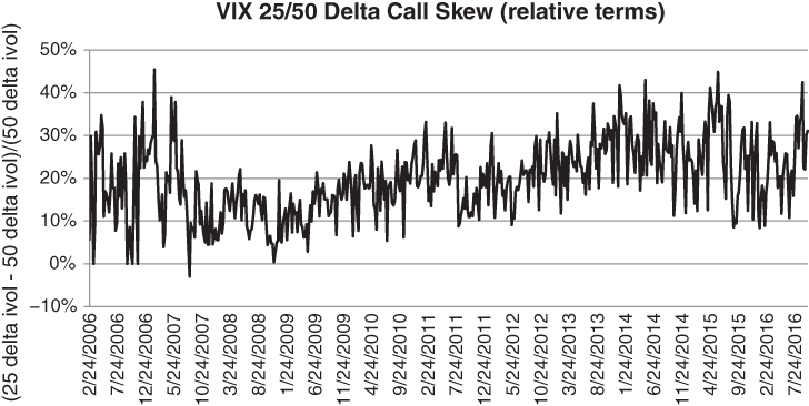Figure 4.36 VIX 25 delta calls have traditionally traded at a large premium to ATM calls

One drawback of the short futures/long call strategy has to do with margining. Since VIX futures trade at a different exchange from VIX options, offsetting legs need to be margined separately. This increases the amount of equity needed to finance the hedge. A reasonable alternative is to sell VXX ETF shares short, while buying VXX calls. However, we have to accept that the ETF will have a variable borrow cost and the calls may be less liquid than their VIX counterparts.

REFLECTIONS ON FIGURE 4.36

Figure 4.36 demonstrates that our strategy has a strong convex payout based on changes in the VIX. It particularly benefits from large moves in the futures. The quadratic regression shows the convex properties of the strategy. The regression has the form , with an R2 of roughly 0.25. Here, a, b and c are greater than 0. You shouldn't be fooled into thinking that, since the intercept is negative, our strategy has negative alpha. The “true” alpha of the strategy is probably close to 0 and materially positive in terms of its impact on a portfolio. The standard alpha interpretation only applies to linear regressions. A one factor linear regression takes the form . We can think of x as the returns for a benchmark and y as the returns of an active manager who tracks the benchmark. is the y-intercept of the regression, the place where the regression line crosses the y-axis. In the language of factor models, it also measures a manager's skill. If is bigger than 0, the implication is that the manager can generate positive returns without market exposure. For quadratic or higher-order regressions, this interpretation is inadequate. Our strategy clearly has a non-linear dependence on changes in the VIX. The strategy performs particularly well for large moves in the VIX, no matter what direction. Conversely, it underperforms if there is no move in the underlying. This is the implicit statistical charge you pay for the hedge.

Imagine that we constructed an options position whose payout was (S(T) – S(t))2 – C, where C >= 0. The intercept is negative by construction and the payout function resembles a long straddle. If S(T) lands at S(t), you lose –C on the trade. However, assuming C is small enough and S(T) has non-0 volatility, the expected payout of the position must be positive. This corresponds to the notion that there must be some price where an option is underpriced, as long as the spot volatility is greater than 0. Based on a standard linear regression, we generate a positive intercept, namely with .

It remains to justify why we can be so confident that this structure will provide protection during a severe drawdown in the S&P 500. Recall that we have cautioned against relying too much on cross-asset class correlations when constructing a hedge. In some cases, the indirect hedge is relatively safe, if not foolproof. In others, the banked-upon correlation can disappear when you need it the most. Offsetting exposure to one risky asset with puts on another tends to work most of the time. For example, it seems reasonable to buy S&P 500 puts to hedge European equity and credit risk, on the assumption that US implied volatility is relatively cheap. In this way, you can minimise the cost of hedging against a systemic risk event. However, buying calls on a random asset that has historically been negatively correlated to your core portfolio is potentially dangerous. Treasury bonds are the canonical example. Treasuries have rallied during equity sell-offs over the past 30 years, implying persistent negative correlation. However, in a highly inflationary environment, there is no guarantee that they should do so. We refer to Illmanen (2003) for a detailed discussion of this subtlety. Given our reservations, do VIX calls offer a rock solid hedge against equity risk? After all, they are playing the role of the negatively correlated asset. We would argue that they do, as the VIX and S&P 500 are structurally linked (see Figure 4.37). VIX calls don't directly protect against adverse moves in the S&P. However, the VIX directly measures the price of insurance on the index. This implies that VIX calls will protect against an increase in the price of S&P 500 puts, should you decide to buy protection later. The linkage between the performance of VIX calls and the magnitude of S&P sell-offs is strong. The mechanical connection between the VIX and S&P implies that there is likely to be a large negative correlation between the VIX and the S&P over the longterm, as there has been in the past. 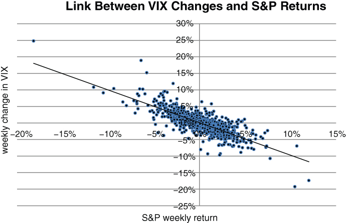Figure 4.37 Strong structural linkage between VIX changes and S&P returns

MIGRATING TO DIFFERENT MARKETS: THE V2X

We have shown how to construct VIX options structures that provide significant protection against a risk event, while minimising negative carry. Can we apply the same technique to other volatility indices, such as the V2X? In theory, we could diversify our hedging overlays by venturing into other markets. Note that the V2X is the analogue of the VIX for the Euro Stoxx 50 index. As of this writing, the V2X doesn't trade nearly as efficiently as the VIX. This makes hedging difficult. Front month V2X futures provide reasonably accurate protection against severe drops in the Euro Stoxx 50 index. However, neither the options nor the futures market is very developed or liquid. This restricts the range of possible hedges. For example, there has been a December dip or kink in the V2X futures term structure for the past several years, as in the Figure 4.38. 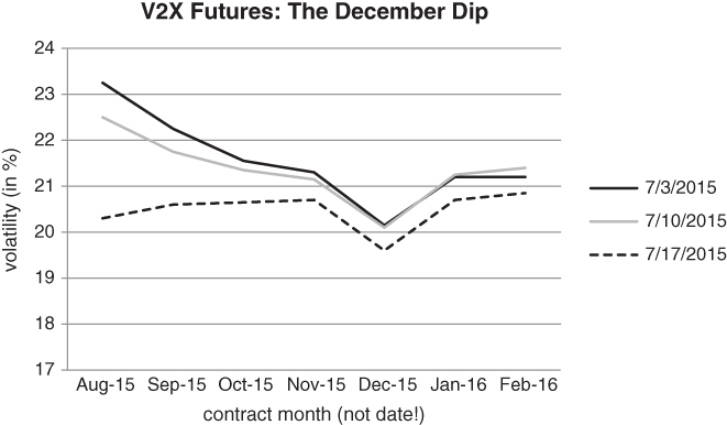Figure 4.38 Santa sells V2X futures while attempting to buy global equities

The December dip in the term structure is terribly annoying. It feels like an itch that you can't scratch. The temptation is to try to trade away the Santa dip. An obvious idea would be to buy the Nov/Dec/Jan butterfly, buying 2 December futures while selling one each of November and January. This trade would be profitable as soon as the dip disappeared. You would disproportionately profit from the Santa V2X contract. Yield curves generally do not have seasonal dips in them. You can only argue in favour of a dip if realised volatility in December is expected to be dramatically below volatility in the surrounding months. The VIX term structure has no such irregularities, as you can see in Figure 4.39. 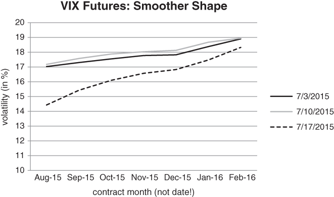Figure 4.39 By comparison, the December dip in VIX futures is modest

This implies that if you need to hedge a long portfolio of European stocks, you might be better off using VIX options. While the VIX hedge is clearly less specific, it should behave more predictably during a major risk event. Different strikes and maturities are likely to behave in a coordinated way. You need to find a balance between specificity, predictability and cost in any hedging mandate. As of this writing, the V2X is too unpredictable to strike this balance correctly.

RISK-REGIME ANALYSIS

We have harped on about the “every dog has its day” theme several times in this book. Every option structure has its moment to shine. Even a silly looking combination of options will pay out admirably in the right scenario. Some hedges outperform in quiet markets, while others offer relatively good value once volatility picks up. How can we quantify the conditional performance of various options strategies? We first need a regime indicator, which specifies the state of the market at any given time. We might not have any idea where we are going, but at least we know where we are on the map now. Then, we can tabulate the performance of each hedging structure based on the prevailing regime. This approach allows us to select reasonable hedges no matter what is going on in the market. From our perspective, hedges that offer decent value in “risk off” phases are particularly valuable. These might be the best defensive strategies after the market has already started to sell off. In short, they satisfy our “second leg down” imperative.

In this section, we construct a simple regime indicator and use it to condition the performance of the hedges we have described above. We use the VIX as a proxy for global asset class risk. Whenever the VIX is sufficiently above its 3-year historical average, we say that the market is “risk off”. Otherwise, the market is said to be “risk on”. Risk off phases are characterised by declining equity indices, widening credit spreads and increased FX volatility. Conversely, “risk on” refers to a benign market that is either rising or not moving around very much. As in Malek (2009), we have calibrated our regime indicator so that it spends more time in risk on phases than risk off ones. This seems intuitively correct. You want to spend more time invested in the market than sitting in cash. Markets do tend to go up, most of the time. You want to harvest the risk premia that are available, while avoiding potential disaster. There is a saying that goes “time in the market is more important than timing the market”. While this might seem like self-indulgent word play, it applies here. Imagine that you were a long-only US equity fund manager, but had to sit in cash 75% of the time. You would need exceptional timing to come anywhere close to the index over a reasonable horizon, assuming the index had positive drift. By contrast, according to this approach, you don't want to be hanging around when things are looking ominous. If you manage to avoid the devastating drawdowns that occur infrequently but are in the market most other times, you may have a recipe for outperformance. This turns the problem of generating alpha on its head. Market beta is now your source of passive return, while risk management produces alpha. The idea is to make your money while the going is good and get out when things deteriorate.

This is a reasonable approach, on the assumption that risky assets go up most of the time. However, every now and again their progress is halted by sharp sell-offs or protracted bear markets. Malek (2009) uses a broader risk indicator than the VIX to tabulate the regime-based performance of various hedge fund strategies. This indicator was more comprehensive, in an attempt to deal with situations where volatility moves asynchronously across interest rates, currencies and equity indices. But is such complexity necessary? It is worth checking whether the VIX is sufficient as a risk indicator, for two reasons. When we classify the performance of various hedging strategies according to regime, we want to verify that our conclusions are not too sensitive to the choice of indicator. The last thing we want is a highly complicated risk index that optimises over a large number of indices, as it is less likely to be reliable. But there is another, more important, reason for advocating simplicity. We want to convince ourselves that, during a severe crisis, it doesn't really matter where you hedge. We have already argued that consultants tend to be overly focused on precise hedges, when something cheap that does the job in a crisis might be preferable. However, we haven't offered much evidence for this assertion. Our thesis is that you can buy puts on risky currencies, equities or high yielding bonds. All are fair game. In extreme market conditions, implied volatility across risky asset classes will be intertwined. If true, you can focus on finding inexpensive hedges across asset classes, without excessive concern for the most precise hedge. Figure 4.40 demonstrates that weekly changes in benchmark equity and currency implied volatility have a strong statistical correlation. 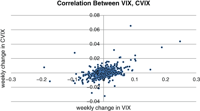Figure 4.40 Weekly changes in currency and equity index implied volatility are inter-linked

In Figure 4.41, we verify that the VIX is indeed a sufficient risk indicator. It might not capture all of the subtleties of market sell-offs, but it adequately flags the worst ones. We start with three implied volatility indices: the VIX, the CVIX and the MOVE index, one for equities, one for currencies and one for bonds. The VIX is a measure of US equity index risk. The CVIX is the currency analogue of the VIX, for currencies. It measures 3-month implied volatility for an aggregate of 9 major currency pairs, with a relatively large allocation to the EUR/USD, USD/JPY and GBP/USD crosses. The MOVE index is a weighted average of 1-month implied volatility for constant maturity 2-, 5-, 10- and 30-year US Treasury bonds. Recall that a constant maturity “bond” doesn't correspond to a specific bond, but is constructed from a weighted average of bond yields near the maturity target. We then calculate the 3-year trailing Z score of each index. The Z score simply measures how many standard deviations the index is away from its average. If an index has a Z score of 2, it is 2 standard deviations higher than normal. This is a significant difference, indicating that the index is severely elevated. 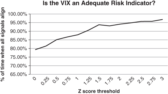Figure 4.41 The CVIX, MOVE and VIX indices become increasingly correlated as the VIX rises

Having calculated the Z score of the VIX, CVIX and MOVE, we can check whether each index triggers a “risk off” signal at the same time. In particular, we choose a threshold, then ask the following question. If the Z score of the VIX is above the threshold, are the Z scores of the CVIX and MOVE also above the threshold? If so, the CVIX and MOVE are simply confirming what the VIX already has to say. It turns out that, as the threshold rises, the 3 volatility indices are nearly always in agreement. For example, whenever the VIX is more than 2 standard deviations above normal, the CVIX and MOVE will also be more than 2 standard deviations above normal roughly 95% of the time.

It's also important to verify that the CVIX doesn't spike without confirmation from the VIX. We don't want the set of instances where one risk indicator spikes to be much larger than the set of instances where the others do. This would imply that the VIX (say) might miss significant “risk off” events in the currency markets. In Figure 4.42, we swap the CVIX for the VIX and re-apply the threshold test. 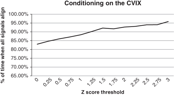Figure 4.42 When the CVIX is high, the MOVE and VIX indices tend to be switched on as well

CONDITIONAL PERFORMANCE OF HEDGING STRATEGIES

In the absence of a mega event, buying and selling fixed delta options is a losing strategy over the long term. With this in mind, we want to identify strikes that are best suited to particular market regimes. In Figure 4.44, we graph our binary VIX-derived risk index. “Risk on” and “risk off” phases are denoted by +1 and –1, respectively. When the market is risk on, investors are driven more by greed than fear. They want to buy equities and credit, while selling volatility. Conversely, risk off phases span the range of emotions from cautiousness to abject fear. 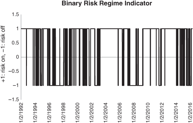Figure 4.43 Our international bar code risk indicator 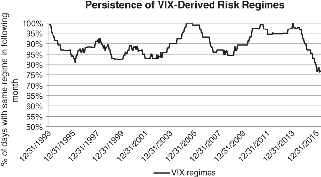Figure 4.44 Decline in risk regime persistence since 2013

Note that we have calculated the 2-year trailing Z score of the VIX and mapped it to +1 whenever the Z score was below 0.5 and –1 otherwise. This creates a binary signal that is biased toward “risk on” phases. We want risk on phases to be more frequent than risk off ones, based on the observation that quiet (bull) markets typically last longer than turbulent (bear) ones. Assuming that the Z-score series is reasonably normally distributed with 0 mean, the 0.5 threshold implies that the market will be risk “on” about 70% of the time.

A regime-based approach to strategy selection should intuitively work best when there is not too much switching from +1 to –1. More succinctly, we want persistence in the index. This allows us to overweight strategies that typically perform well in the current regime, with reasonable confidence that the regime will not change at a moment's notice. Figure 4.44 uses a moving 2-year window to calculate the frequency with which the prevailing regime stays constant from one week to the next.

The index is generally quite sticky, implying that allocating to strategies that have performed well in the current regime is a reasonable long-term idea. However, there has been a notable dip in persistence since the end of 2013. This suggests that investors have been relatively schizophrenic in their desire to take risk, swinging from greed to fear with high frequency.

Our risk index allows us to draw some conclusions about the appropriate hedge for a given market regime. It formalises the “every dog has its day” approach to options strategies. Figure 4.45 summarises the average weekly performance of 1-month S&P puts with various deltas, conditional on regime. We have normalised the returns of the 10, 25 and 40 delta put buying strategies so that their in-sample volatility matches the 50 delta put volatility. For example, we need to buy more 10 delta puts than 25 delta puts if we want their realised volatility to match. The black bars show average performance if the previous week was risk off. The grey ones are based on those occasions where the previous week was risk on. It's not surprising that the black bars are lower than the grey ones, as the cost of hedging increases after volatility jumps. 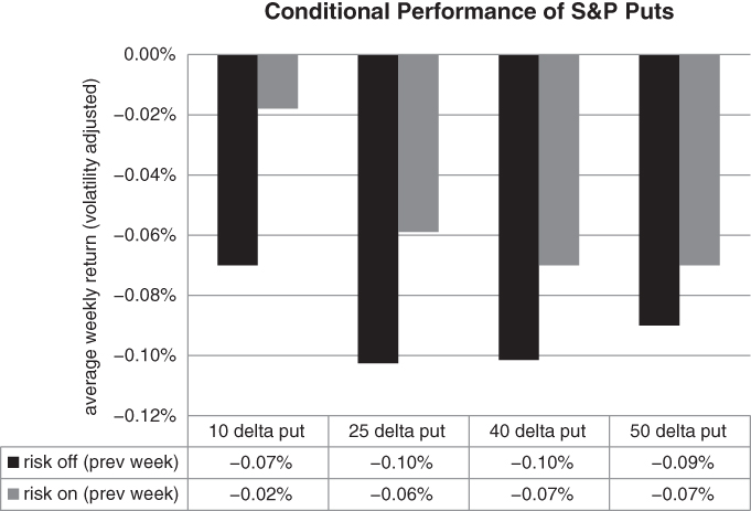Figure 4.45 Relative performance of variable delta puts, conditioned on risk regime from previous week

We want to know whether the current regime gives us a clue as to what to do next.

The 10 delta S&P put has outperformed in both regimes over the past 10 years. Even on a volatility adjusted basis, it has declined at a shallower pace than a rolling strategy with higher delta puts. The difference is especially large during risk on periods. Another observation is that the 10 delta puts (volatility adjusted) are superior to the 25 delta puts in both regimes. This suggests that a short 1×2 put ratio spread, with 25 and 10 delta strikes is a reasonable “all weather” strategy, as we have previously discussed. The square root payout has merit from an unconditional statistical standpoint. However, the 1×2 is particularly compelling when the market is risk on. This may be an issue of cost. 10 delta puts seem to offer good relative value in quiet markets as the put skew tends to be relatively flat when investors are feeling buoyant.

We can conduct the same analysis for VXX calls as shown in Figure 4.46. The VXX is an exchange-traded fund, or “ETF”, that tries to replicate the performance of a rolling strategy in short-term VIX futures. Options data for the VXX only goes back to 2010, so we have to content ourselves with a fairly short study. Alternatively, we could try to analyse VIX options with various deltas allowing us to go back a bit further in time. However, testing a VIX options strategy can be treacherous. We would need to calculate the VIX forward price that precisely matches the time to maturity of a given call or else our Black–Scholes implied volatilities would be mis-specified. 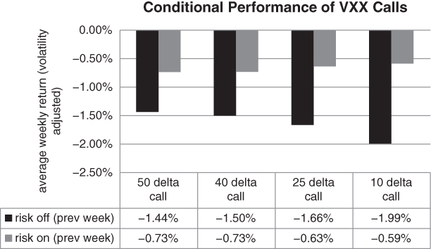Figure 4.46 Conditional performance of VXX calls with variable deltas

As in Figure 4.45, we have matched the volatility of each call buying strategy. Here, the results are less overwhelmingly in favour of a single delta. The 50 delta put seems to function best in risk off environments, while the 10 delta call is best suited for risk on ones. Investors have a tendency to overprice the OTM call skew when VIX implied volatility spikes.

SUMMARY

Several important conclusions can be drawn from this chapter.

• Deep out-of-the-money puts on equity indices generally offer superior value to the mildly OTM puts that institutions favour.
• You can take advantage of institutional bias by selling put ratio spreads, i.e. selling a small number of overpriced OTM puts to finance the purchase of a large number of deep OTM puts.
• The short ratio spread can give you levered long exposure to the implied volatility skew in advance of a crisis, at low cost.
• While the VIX is theoretically attractive as a portfolio hedge, implementation is a major hurdle. You either face severe roll down or mean reversion when buying VIX futures. VIX call options face the added obstacle of time decay. It is extremely difficult to recreate the spot VIX in practice.
• A reasonable alternative involves simultaneously selling VIX futures and overbuying ATM VIX calls. This dramatically reduces exposure to roll down while providing a convex payout on implied volatility. In other words, the structure benefits from large changes in volatility in either direction.
• The VIX futures/call strategy can be useful in risk off regimes, after volatility has risen. It is a useful second leg down strategy if you believe that volatility is likely to slingshot away from its current level.